Agfdhyk

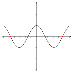
A graph of the function cos⁡(x){displaystyle cos(x)} for x{displaystyle x} in [−2π,2π]{displaystyle left[-2pi ,2pi right]}, with zeros at −3π2,−π2,π2{displaystyle -{tfrac {3pi }{2}},;-{tfrac {pi }{2}},;{tfrac {pi }{2}}}, and 3π2,{displaystyle {tfrac {3pi }{2}},} marked in red.

In mathematics, a zero, also sometimes called a root, of a real-, complex- or generally vector-valued function f{displaystyle f} is a member x{displaystyle x} of the domain of f{displaystyle f} such that f(x){displaystyle f(x)} vanishes at x{displaystyle x}; that is, x{displaystyle x} is a solution of the equation f(x)=0{displaystyle f(x)=0}.
In other words, a "zero" of a function is an input value that produces an output of 0{displaystyle 0}.^[1]

A root of a polynomial is a zero of the corresponding polynomial function.
The fundamental theorem of algebra shows that any non-zero polynomial has a number of roots at most equal to its degree and that the number of roots and the degree are equal when one considers the complex roots (or more generally the roots in an algebraically closed extension) counted with their multiplicities. For example, the polynomial f{displaystyle f} of degree two, defined by

f(x)=x2−5x+6{displaystyle f(x)=x^{2}-5x+6}

has the two roots 2{displaystyle 2} and 3{displaystyle 3}, since

f(2)=22−5⋅2+6=0andf(3)=32−5⋅3+6=0{displaystyle f(2)=2^{2}-5cdot 2+6=0quad {textrm {and}}quad f(3)=3^{2}-5cdot 3+6=0}.

If the function maps real numbers to real numbers, its zeros are the x{displaystyle x}-coordinates of the points where its graph meets the x-axis. An alternative name for such a point (x,0){displaystyle (x,0)} in this context is an x{displaystyle x}-intercept.

Solution of an equation

Every equation in the unknown x may be rewritten as

f(x)=0{displaystyle f(x)=0}

by regrouping all terms in the left-hand side. It follows that the solutions of such an equation are exactly the zeros of the function f{displaystyle f}. In other words, "zero of a function" is a phrase denoting a "solution of the equation obtained by equating the function to 0," and the study of zeros of functions is exactly the same as the study of solutions of equations.

Polynomial roots

Every real polynomial of odd degree has an odd number of real roots (counting multiplicities); likewise, a real polynomial of even degree must have an even number of real roots. Consequently, real odd polynomials must have at least one real root (because one is the smallest odd whole number), whereas even polynomials may have none. This principle can be proven by reference to the intermediate value theorem: since polynomial functions are continuous, the function value must cross zero in the process of changing from negative to positive or vice versa.

Fundamental theorem of algebra

The fundamental theorem of algebra states that every polynomial of degree n{displaystyle n} has n{displaystyle n} complex roots, counted with their multiplicities. The non-real roots of polynomials with real coefficients come in conjugate pairs.^[1]Vieta's formulas relate the coefficients of a polynomial to sums and products of its roots.

Computing roots

Computing roots of functions, for example polynomial functions, frequently requires the use of specialised or approximation techniques (for example, Newton's method). However, some polynomial functions, including all those of degree no greater than 4, can have all their roots expressed algebraically in terms of their coefficients. (See algebraic solution.)

Zero set

In various areas of mathematics, the zero set of a function is the set of all its zeros. More precisely, if f:X→R{displaystyle f:Xto mathbb {R} } is a real-valued function (or, more generally, a function taking values in some additive group), its zero set is f−1(0){displaystyle f^{-1}(0)} of X{displaystyle X}, the inverse image of {0}{displaystyle {0}}).

The term zero set is generally used when there are infinitely many zeros, and they have some non-trivial topological properties. For example, a level set of a function f{displaystyle f} is the zero set of f−c{displaystyle f-c}. The cozero set of f{displaystyle f} is the complement of the zero set of f{displaystyle f} (i.e., the subset of X{displaystyle X} on which f{displaystyle f} is nonzero).

Applications

In algebraic geometry, the first definition of an algebraic variety is through zero sets. Specifically, an affine algebraic set is the intersection of the zero sets of several polynomials in a polynomial ring k[x1,…,xn]{displaystyle kleft[x_{1},ldots ,x_{n}right]} over a field. In this context, a zero set is sometimes called a zero locus.

In analysis and geometry, any closed subset of Rn{displaystyle mathbb {R} ^{n}} is the zero set of a smooth function defined on all of Rn{displaystyle mathbb {R} ^{n}}. This extends to any smooth manifold as a corollary of paracompactness.

In differential geometry, zero sets are frequently used to define manifolds. An important special case is the case that f{displaystyle f} is a smooth function from Rp{displaystyle mathbb {R} ^{p}} to Rn{displaystyle mathbb {R} ^{n}}. If zero is a regular value of f{displaystyle f}, then the zero set of f{displaystyle f} is a smooth manifold of dimension m=p−n{displaystyle m=p-n} by the regular value theorem.

For example, the unit m{displaystyle m}-sphere in Rm+1{displaystyle mathbb {R} ^{m+1}} is the zero set of the real-valued function f(x)=|x|2−1{displaystyle f(x)=vert xvert ^{2}-1}.

See also

• Zeros and poles


• Sendov's conjecture


• Marden's theorem


• Vanish at infinity


• Zero crossing

References

Further reading

• Weisstein, Eric W. "Root". MathWorld.

References

^ ab Foerster, Paul A. (2006). Algebra and Trigonometry: Functions and Applications, Teacher's Edition (Classics ed.). Upper Saddle River, NJ: Prentice Hall. p. 535. ISBN 0-13-165711-9..mw-parser-output cite.citation{font-style:inherit}.mw-parser-output q{quotes:"""""""'""'"}.mw-parser-output code.cs1-code{color:inherit;background:inherit;border:inherit;padding:inherit}.mw-parser-output .cs1-lock-free a{background:url("//upload.wikimedia.org/wikipedia/commons/thumb/6/65/Lock-green.svg/9px-Lock-green.svg.png")no-repeat;background-position:right .1em center}.mw-parser-output .cs1-lock-limited a,.mw-parser-output .cs1-lock-registration a{background:url("//upload.wikimedia.org/wikipedia/commons/thumb/d/d6/Lock-gray-alt-2.svg/9px-Lock-gray-alt-2.svg.png")no-repeat;background-position:right .1em center}.mw-parser-output .cs1-lock-subscription a{background:url("//upload.wikimedia.org/wikipedia/commons/thumb/a/aa/Lock-red-alt-2.svg/9px-Lock-red-alt-2.svg.png")no-repeat;background-position:right .1em center}.mw-parser-output .cs1-subscription,.mw-parser-output .cs1-registration{color:#555}.mw-parser-output .cs1-subscription span,.mw-parser-output .cs1-registration span{border-bottom:1px dotted;cursor:help}.mw-parser-output .cs1-hidden-error{display:none;font-size:100%}.mw-parser-output .cs1-visible-error{font-size:100%}.mw-parser-output .cs1-subscription,.mw-parser-output .cs1-registration,.mw-parser-output .cs1-format{font-size:95%}.mw-parser-output .cs1-kern-left,.mw-parser-output .cs1-kern-wl-left{padding-left:0.2em}.mw-parser-output .cs1-kern-right,.mw-parser-output .cs1-kern-wl-right{padding-right:0.2em}