Agfdhyk

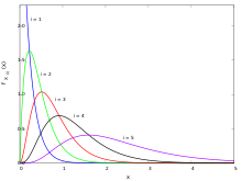
Probability density functions of the order statistics for a sample of size n = 5 from an exponential distribution with unit scale parameter.

In statistics, the kth order statistic of a statistical sample is equal to its kth-smallest value.^[1] Together with rank statistics, order statistics are among the most fundamental tools in non-parametric statistics and inference.

Important special cases of the order statistics are the minimum and maximum value of a sample, and (with some qualifications discussed below) the sample median and other sample quantiles.

When using probability theory to analyze order statistics of random samples from a continuous distribution, the cumulative distribution function is used to reduce the analysis to the case of order statistics of the uniform distribution.

Notation and examples

For example, suppose that four numbers are observed or recorded, resulting in a sample of size 4. If the sample values are

6, 9, 3, 8,

they will usually be denoted

x1=6,  x2=9,  x3=3,  x4=8,{displaystyle x_{1}=6, x_{2}=9, x_{3}=3, x_{4}=8,,}

where the subscript i in xi{displaystyle x_{i}} indicates simply the order in which the observations were recorded and is usually assumed not to be significant. A case when the order is significant is when the observations are part of a time series.

The order statistics would be denoted

x(1)=3,  x(2)=6,  x(3)=8,  x(4)=9,{displaystyle x_{(1)}=3, x_{(2)}=6, x_{(3)}=8, x_{(4)}=9,,}

where the subscript (i) enclosed in parentheses indicates the ith order statistic of the sample.

The first order statistic (or smallest order statistic) is always the minimum of the sample, that is,

X(1)=min{X1,…,Xn}{displaystyle X_{(1)}=min{,X_{1},ldots ,X_{n},}}

where, following a common convention, we use upper-case letters to refer to random variables, and lower-case letters (as above) to refer to their actual observed values.

Similarly, for a sample of size n, the nth order statistic (or largest order statistic) is the maximum, that is,

X(n)=max{X1,…,Xn}.{displaystyle X_{(n)}=max{,X_{1},ldots ,X_{n},}.}

The sample range is the difference between the maximum and minimum. It is a function of the order statistics:

Range{X1,…,Xn}=X(n)−X(1).{displaystyle {rm {Range}}{,X_{1},ldots ,X_{n},}=X_{(n)}-X_{(1)}.}

A similar important statistic in exploratory data analysis that is simply related to the order statistics is the sample interquartile range.

The sample median may or may not be an order statistic, since there is a single middle value only when the number n of observations is odd. More precisely, if n = 2m+1 for some integer m, then the sample median is X(m+1){displaystyle X_{(m+1)}} and so is an order statistic. On the other hand, when n is even, n = 2m and there are two middle values, X(m){displaystyle X_{(m)}} and X(m+1){displaystyle X_{(m+1)}}, and the sample median is some function of the two (usually the average) and hence not an order statistic. Similar remarks apply to all sample quantiles.

Probabilistic analysis

Given any random variables X₁, X₂..., X_n, the order statistics X₍₁₎, X₍₂₎, ..., X_(n) are also random variables, defined by sorting the values (realizations) of X₁, ..., X_n in increasing order.

When the random variables X₁, X₂..., X_n form a sample they are independent and identically distributed. This is the case treated below. In general, the random variables X₁, ..., X_n can arise by sampling from more than one population. Then they are independent, but not necessarily identically distributed, and their joint probability distribution is given by the Bapat–Beg theorem.

From now on, we will assume that the random variables under consideration are continuous and, where convenient, we will also assume that they have a probability density function (PDF), that is, they are absolutely continuous. The peculiarities of the analysis of distributions assigning mass to points (in particular, discrete distributions) are discussed at the end.

Probability distributions of order statistics

Order statistics sampled from a uniform distribution

In this section we show that the order statistics of the uniform distribution on the unit interval have marginal distributions belonging to the Beta distribution family. We also give a simple method to derive the joint distribution of any number of order statistics, and finally translate these results to arbitrary continuous distributions using the cdf.

We assume throughout this section that X1,X2,…,Xn{displaystyle X_{1},X_{2},ldots ,X_{n}} is a random sample drawn from a continuous distribution with cdf FX{displaystyle F_{X}}. Denoting Ui=FX(Xi){displaystyle U_{i}=F_{X}(X_{i})} we obtain the corresponding random sample U1,…,Un{displaystyle U_{1},ldots ,U_{n}} from the standard uniform distribution. Note that the order statistics also satisfy U(i)=FX(X(i)){displaystyle U_{(i)}=F_{X}(X_{(i)})}.

The probability density function of the order statistic U(k){displaystyle U_{(k)}} is equal to^[2]

fU(k)=n!(k−1)!(n−k)!uk−1(1−u)n−k{displaystyle f_{U_{(k)}}={n! over (k-1)!(n-k)!}u^{k-1}(1-u)^{n-k}}

that is, the kth order statistic of the uniform distribution is a beta-distributed random variable.^[2][3]

U(k)∼Beta(k,n+1−k).{displaystyle U_{(k)}sim Beta(k,n+1-k).}

The proof of these statements is as follows. For U(k){displaystyle U_{(k)}} to be between u and u + du, it is necessary that exactly k − 1 elements of the sample are smaller than u, and that at least one is between u and u + du. The probability that more than one is in this latter interval is already O(du2){displaystyle O(du^{2})}, so we have to calculate the probability that exactly k − 1, 1 and n − k observations fall in the intervals (0,u){displaystyle (0,u)}, (u,u+du){displaystyle (u,u+du)} and (u+du,1){displaystyle (u+du,1)} respectively. This equals (refer to multinomial distribution for details)

n!(k−1)!(n−k)!uk−1⋅du⋅(1−u−du)n−k{displaystyle {n! over (k-1)!(n-k)!}u^{k-1}cdot ducdot (1-u-du)^{n-k}}

and the result follows.

The mean of this distribution is k / (n + 1).

The joint distribution of the order statistics of the uniform distribution

Similarly, for i < j, the joint probability density function of the two order statistics U_(i) < U_(j) can be shown to be

fU(i),U(j)(u,v)=n!ui−1(i−1)!(v−u)j−i−1(j−i−1)!(1−v)n−j(n−j)!{displaystyle f_{U_{(i)},U_{(j)}}(u,v)=n!{u^{i-1} over (i-1)!}{(v-u)^{j-i-1} over (j-i-1)!}{(1-v)^{n-j} over (n-j)!}}

which is (up to terms of higher order than O(dudv){displaystyle O(du,dv)}) the probability that i − 1, 1, j − 1 − i, 1 and n − j sample elements fall in the intervals (0,u){displaystyle (0,u)}, (u,u+du){displaystyle (u,u+du)}, (u+du,v){displaystyle (u+du,v)}, (v,v+dv){displaystyle (v,v+dv)}, (v+dv,1){displaystyle (v+dv,1)} respectively.

One reasons in an entirely analogous way to derive the higher-order joint distributions. Perhaps surprisingly, the joint density of the n order statistics turns out to be constant:

fU(1),U(2),…,U(n)(u1,u2,…,un)=n!.{displaystyle f_{U_{(1)},U_{(2)},ldots ,U_{(n)}}(u_{1},u_{2},ldots ,u_{n})=n!.}

One way to understand this is that the unordered sample does have constant density equal to 1, and that there are n! different permutations of the sample corresponding to the same sequence of order statistics. This is related to the fact that 1/n! is the volume of the region 0<u1<⋯<un<1{displaystyle 0<u_{1}<cdots <u_{n}<1}.

Order statistics sampled from an exponential distribution

For X1,X2,..,Xn{displaystyle X_{1},X_{2},..,X_{n}} random samples from an exponential distribution with parameter λ the order statistics X_(i) for i = 1,2,3, ..., n each have distribution

X(i)=d1λ(∑j=1iZjn−j+1){displaystyle X_{(i)}{stackrel {d}{=}}{frac {1}{lambda }}left(sum _{j=1}^{i}{frac {Z_{j}}{n-j+1}}right)}

where the Z_j are iid standard exponential random variables (i.e. with rate parameter 1). This result was first published by Alfréd Rényi.^[4][5]

Order statistics sampled from an Erlang distribution

The Laplace transform of order statistics sampled from an Erlang distribution via a path counting method.^[6]

The joint distribution of the order statistics of an absolutely continuous distribution

If F_X is absolutely continuous, it has a density such that dFX(x)=fX(x)dx{displaystyle dF_{X}(x)=f_{X}(x),dx}, and we can use the substitutions

u=FX(x){displaystyle u=F_{X}(x)}

and

du=fX(x)dx{displaystyle du=f_{X}(x),dx}

to derive the following probability density functions for the order statistics of a sample of size n drawn from the distribution of X:

fX(k)(x)=n!(k−1)!(n−k)![FX(x)]k−1[1−FX(x)]n−kfX(x){displaystyle f_{X_{(k)}}(x)={frac {n!}{(k-1)!(n-k)!}}[F_{X}(x)]^{k-1}[1-F_{X}(x)]^{n-k}f_{X}(x)}

fX(j),X(k)(x,y)=n!(j−1)!(k−j−1)!(n−k)![FX(x)]j−1[FX(y)−FX(x)]k−1−j[1−FX(y)]n−kfX(x)fX(y){displaystyle f_{X_{(j)},X_{(k)}}(x,y)={frac {n!}{(j-1)!(k-j-1)!(n-k)!}}[F_{X}(x)]^{j-1}[F_{X}(y)-F_{X}(x)]^{k-1-j}[1-F_{X}(y)]^{n-k}f_{X}(x)f_{X}(y)} where x≤y{displaystyle xleq y}

fX(1),…,X(n)(x1,…,xn)=n!fX(x1)⋯fX(xn){displaystyle f_{X_{(1)},ldots ,X_{(n)}}(x_{1},ldots ,x_{n})=n!f_{X}(x_{1})cdots f_{X}(x_{n})} where x1≤x2≤⋯≤xn.{displaystyle x_{1}leq x_{2}leq dots leq x_{n}.}

Application: confidence intervals for quantiles

An interesting question is how well the order statistics perform as estimators of the quantiles of the underlying distribution.

A small-sample-size example

The simplest case to consider is how well the sample median estimates the population median.

As an example, consider a random sample of size 6. In that case, the sample median is usually defined as the midpoint of the interval delimited by the 3rd and 4th order statistics. However, we know from the preceding discussion that the probability that this interval actually contains the population median is

(63)2−6=516≈31%.{displaystyle {6 choose 3}2^{-6}={5 over 16}approx 31%.}

Although the sample median is probably among the best distribution-independent point estimates of the population median, what this example illustrates is that it is not a particularly good one in absolute terms. In this particular case, a better confidence interval for the median is the one delimited by the 2nd and 5th order statistics, which contains the population median with probability

[(62)+(63)+(64)]2−6=2532≈78%.{displaystyle left[{6 choose 2}+{6 choose 3}+{6 choose 4}right]2^{-6}={25 over 32}approx 78%.}

With such a small sample size, if one wants at least 95% confidence, one is reduced to saying that the median is between the minimum and the maximum of the 6 observations with probability 31/32 or approximately 97%. Size 6 is, in fact, the smallest sample size such that the interval determined by the minimum and the maximum is at least a 95% confidence interval for the population median.

Large sample sizes

For the uniform distribution, as n tends to infinity, the p^th sample quantile is asymptotically normally distributed, since it is approximated by

U(⌈np⌉)∼AN(p,p(1−p)n).{displaystyle U_{(lceil nprceil )}sim ANleft(p,{frac {p(1-p)}{n}}right).}

For a general distribution F with a continuous non-zero density at F ⁻¹(p), a similar asymptotic normality applies:

X(⌈np⌉)∼AN(F−1(p),p(1−p)n[f(F−1(p))]2){displaystyle X_{(lceil nprceil )}sim ANleft(F^{-1}(p),{frac {p(1-p)}{n[f(F^{-1}(p))]^{2}}}right)}

where f is the density function, and F ⁻¹ is the quantile function associated with F. One of the first people to mention and prove this result was Frederick Mosteller in his seminal paper in 1946.^[7] Further research lead in the 1960s to the Bahadur representation which provides information about the errorbounds.

An interesting observation can be made in the case where the distribution is symmetric, and the population median equals the population mean. In this case, the sample mean, by the central limit theorem, is also asymptotically normally distributed, but with variance σ²/n instead. This asymptotic analysis suggests that the mean outperforms the median in cases of low kurtosis, and vice versa. For example, the median achieves better confidence intervals for the Laplace distribution, while the mean performs better for X that are normally distributed.

Proof

It can be shown that

B(k,n+1−k) =d XX+Y,{displaystyle B(k,n+1-k) {stackrel {mathrm {d} }{=}} {frac {X}{X+Y}},}

where

X=∑i=1kZi,Y=∑i=k+1n+1Zi,{displaystyle X=sum _{i=1}^{k}Z_{i},quad Y=sum _{i=k+1}^{n+1}Z_{i},}

with Z_i being independent identically distributed exponential random variables with rate 1. Since X/n and Y/n are asymptotically normally distributed by the CLT, our results follow by application of the delta method.

Application: Non-parametric Density Estimation

Moments of the distribution for the first order statistic can be used to develop a non-parametric density estimator.^[8] Suppose, we want to estimate the density fX{displaystyle f_{X}} at the point x∗{displaystyle x^{*}}. Consider the random variables Yi=|Xi−x∗|{displaystyle Y_{i}=|X_{i}-x^{*}|}, which are i.i.d with distribution function gY(y)=fX(y+x∗)+fX(x∗−y){displaystyle g_{Y}(y)=f_{X}(y+x^{*})+f_{X}(x^{*}-y)}. In particular, fX(x∗)=gY(0)2{displaystyle f_{X}(x^{*})={frac {g_{Y}(0)}{2}}}.

The expected value of the first order statistic Y(1){displaystyle Y_{(1)}} given N{displaystyle N} total samples yields,

E(Y(1))=1(N+1)g(0)+1(N+1)(N+2)∫01Q″(z)δN+1(z)dz{displaystyle E(Y_{(1)})={frac {1}{(N+1)g(0)}}+{frac {1}{(N+1)(N+2)}}int _{0}^{1}Q''(z)delta _{N+1}(z),dz}

where Q{displaystyle Q} is the quantile function associated with the distribution gY{displaystyle g_{Y}}, and δN(z)=(N+1)(1−z)N{displaystyle delta _{N}(z)=(N+1)(1-z)^{N}}. This equation in combination with a jackknifing technique becomes the basis for the following density estimation algorithm,

  Input: N{displaystyle N} samples. {xl}l=1M{displaystyle {x_{l}}_{l=1}^{M}} points of density evaluation. Tuning parameter a∈(0,1){displaystyle ain (0,1)} (usually 1/3).

  Output: {f^l}l=1M{displaystyle {{hat {f}}_{l}}_{l=1}^{M}} estimated density at the points of evaluation.

  1: Set mN=round(N1−a){displaystyle m_{N}=round(N^{1-a})}

  2: Set sN=NmN{displaystyle s_{N}={frac {N}{m_{N}}}}

  3: Create an sN×mN{displaystyle s_{N}times m_{N}} matrix Mij{displaystyle M_{ij}} which holds mN{displaystyle m_{N}} subsets with sN{displaystyle s_{N}} samples each.

  4: Create a vector f^{displaystyle {hat {f}}} to hold the density evaluations.

  5: for l=1→M{displaystyle l=1to M} do

  6:     for k=1→mN{displaystyle k=1to m_{N}} do

  7:         Find the nearest distance dlk{displaystyle d_{lk}} to the current point xl{displaystyle x_{l}} within the k{displaystyle k}th subset

  8:      end for

  9:      Compute the subset average of distances to xl:dl=∑k=1mNdlkmN{displaystyle x_{l}:d_{l}=sum _{k=1}^{m_{N}}{frac {d_{lk}}{m_{N}}}}

 10:      Compute the density estimate at xl:f^l=12dl{displaystyle x_{l}:{hat {f}}_{l}={frac {1}{2d_{l}}}}

 11:  end for

 12: return f^{displaystyle {hat {f}}}  

In contrast to the bandwidth/length based tuning parameters for histogram and kernel based approaches, the tuning parameter for the order statistic based density estimator is the size of sample subsets. Such an estimator is more robust than histogram and kernel based approaches, for example densities like the Cauchy distribution (which lack finite moments) can be inferred without the need for specialized modifications such as IQR based bandwidths. This is because the first moment of the order statistic always exists if the expected value of the underlying distribution does, but the converse is not necessarily true.^[9]

Dealing with discrete variables

Suppose X1,X2,...,Xn{displaystyle X_{1},X_{2},...,X_{n}} are i.i.d. random variables from a discrete distribution with cumulative distribution function F(x){displaystyle F(x)} and probability mass function f(x){displaystyle f(x)}. To find the probabilities of the kth{displaystyle k^{text{th}}} order statistics, three values are first needed, namely

p1=P(X<x)=F(x)−f(x), p2=P(X=x)=f(x), and p3=P(X>x)=1−F(x).{displaystyle p_{1}=P(X<x)=F(x)-f(x), p_{2}=P(X=x)=f(x),{text{ and }}p_{3}=P(X>x)=1-F(x).}

The cumulative distribution function of the kth{displaystyle k^{text{th}}} order statistic can be computed by noting that

P(X(k)≤x)=P(there are at most n−k observations greater than or equal to x),=∑j=0n−k(nj)p3j(p1+p2)n−j.{displaystyle {begin{aligned}P(X_{(k)}leq x)&=P({text{there are at most }}n-k{text{ observations greater than or equal to }}x),\&=sum _{j=0}^{n-k}{n choose j}p_{3}^{j}(p_{1}+p_{2})^{n-j}.end{aligned}}}

Similarly, P(X(k)<x){displaystyle P(X_{(k)}<x)} is given by

P(X(k)<x)=P(there are at most n−k observations greater thanx),=∑j=0n−k(nj)(p2+p3)j(p1)n−j.{displaystyle {begin{aligned}P(X_{(k)}<x)&=P({text{there are at most }}n-k{text{ observations greater than}}x),\&=sum _{j=0}^{n-k}{n choose j}(p_{2}+p_{3})^{j}(p_{1})^{n-j}.end{aligned}}}

Note that the probability mass function of Xk{displaystyle X_{k}} is just the difference of these values, that is to say

P(X(k)=x)=P(X(k)≤x)−P(X(k)<x),=∑j=0n−k(nj)(p3j(p1+p2)n−j−(p2+p3)j(p1)n−j),=∑j=0n−k(nj)((1−F(x))j(F(x))n−j−(1−F(x)+f(x))j(F(x)−f(x))n−j).{displaystyle {begin{aligned}P(X_{(k)}=x)&=P(X_{(k)}leq x)-P(X_{(k)}<x),\&=sum _{j=0}^{n-k}{n choose j}left(p_{3}^{j}(p_{1}+p_{2})^{n-j}-(p_{2}+p_{3})^{j}(p_{1})^{n-j}right),\&=sum _{j=0}^{n-k}{n choose j}left((1-F(x))^{j}(F(x))^{n-j}-(1-F(x)+f(x))^{j}(F(x)-f(x))^{n-j}right).end{aligned}}}

Computing order statistics

The problem of computing the kth smallest (or largest) element of a list is called the selection problem and is solved by a selection algorithm. Although this problem is difficult for very large lists, sophisticated selection algorithms have been created that can solve this problem in time proportional to the number of elements in the list, even if the list is totally unordered. If the data is stored in certain specialized data structures, this time can be brought down to O(log n). In many applications all order statistics are required, in which case a sorting algorithm can be used and the time taken is O(n log n).

See also

• Rankit


• Box plot


• Concomitant (statistics)


• Fisher–Tippett distribution


• 
  Bapat–Beg theorem for the order statistics of independent but not necessarily identically distributed random variables


• Bernstein polynomial


• 
  L-estimator – linear combinations of order statistics


• Rank-size distribution


• Selection algorithm

Examples of order statistics

• Sample maximum and minimum


• Quantile


• Percentile


• Decile


• Quartile


• Median

This article includes a list of references, but its sources remain unclear because it has insufficient inline citations. Please help to improve this article by introducing more precise citations. (December 2010) (Learn how and when to remove this template message)

References

• 
  Sefling, R. J. (1980). Approximation Theorems of Mathematical Statistics. New York: Wiley. ISBN 0-471-02403-1.
  

External links

• 
  Order statistics at PlanetMath.org. Retrieved Feb 02,2005


• 
  Weisstein, Eric W. "Order Statistic". MathWorld. Retrieved Feb 02,2005


• Dr. Susan Holmes Order Statistics Retrieved Feb 02,2005


• C++ source Dynamic Order Statistics

References

^ David, H. A.; Nagaraja, H. N. (2003). "Order Statistics". Wiley Series in Probability and Statistics. doi:10.1002/0471722162. ISBN 9780471722168..mw-parser-output cite.citation{font-style:inherit}.mw-parser-output q{quotes:"""""""'""'"}.mw-parser-output code.cs1-code{color:inherit;background:inherit;border:inherit;padding:inherit}.mw-parser-output .cs1-lock-free a{background:url("//upload.wikimedia.org/wikipedia/commons/thumb/6/65/Lock-green.svg/9px-Lock-green.svg.png")no-repeat;background-position:right .1em center}.mw-parser-output .cs1-lock-limited a,.mw-parser-output .cs1-lock-registration a{background:url("//upload.wikimedia.org/wikipedia/commons/thumb/d/d6/Lock-gray-alt-2.svg/9px-Lock-gray-alt-2.svg.png")no-repeat;background-position:right .1em center}.mw-parser-output .cs1-lock-subscription a{background:url("//upload.wikimedia.org/wikipedia/commons/thumb/a/aa/Lock-red-alt-2.svg/9px-Lock-red-alt-2.svg.png")no-repeat;background-position:right .1em center}.mw-parser-output .cs1-subscription,.mw-parser-output .cs1-registration{color:#555}.mw-parser-output .cs1-subscription span,.mw-parser-output .cs1-registration span{border-bottom:1px dotted;cursor:help}.mw-parser-output .cs1-hidden-error{display:none;font-size:100%}.mw-parser-output .cs1-visible-error{font-size:100%}.mw-parser-output .cs1-subscription,.mw-parser-output .cs1-registration,.mw-parser-output .cs1-format{font-size:95%}.mw-parser-output .cs1-kern-left,.mw-parser-output .cs1-kern-wl-left{padding-left:0.2em}.mw-parser-output .cs1-kern-right,.mw-parser-output .cs1-kern-wl-right{padding-right:0.2em}
^ ab Gentle, James E. (2009), Computational Statistics, Springer, p. 63, ISBN 9780387981444.
^ Jones, M. C. (2009), "Kumaraswamy's distribution: A beta-type distribution with some tractability advantages", Statistical Methodology, 6 (1): 70–81, doi:10.1016/j.stamet.2008.04.001,As is well known, the beta distribution is the distribution of the m’th order statistic from a random sample of size n from the uniform distribution (on (0,1)).
^ David, H. A.; Nagaraja, H. N. (2003), "Chapter 2. Basic Distribution Theory", Order Statistics, Wiley Series in Probability and Statistics, p. 9, doi:10.1002/0471722162.ch2, ISBN 9780471722168
^ Rényi, Alfréd (1953). "On the theory of order statistics" (PDF). Acta Mathematica Hungarica. 4 (3): 191–231. doi:10.1007/BF02127580. Archived from the original (PDF) on 2016-10-09.
^ Hlynka, M.; Brill, P. H.; Horn, W. (2010). "A method for obtaining Laplace transforms of order statistics of Erlang random variables". Statistics & Probability Letters. 80: 9. doi:10.1016/j.spl.2009.09.006.
^ Mosteller, Frederick (1946). "On Some Useful "Inefficient" Statistics". Annals of Mathematical Statistics. Institute of Mathematical Statistics. 17 (4): 377–408. doi:10.1214/aoms/1177730881. Retrieved February 26, 2015.
^ Garg, Vikram V.; Tenorio, Luis; Willcox, Karen (2017). "Minimum local distance density estimation". Communications in Statistics-Theory and Methods. 46 (1): 148–164. doi:10.1080/03610926.2014.988260. Retrieved 2019-01-03.
^ David, H. A.; Nagaraja, H. N. (2003), "Chapter 3. Expected Values and Moments", Order Statistics, Wiley Series in Probability and Statistics, p. 34, doi:10.1002/0471722162.ch3, ISBN 9780471722168