Agfdhyk

Part of a series of articles about
Electromagnetism
Electricity Magnetism
Electrostatics Conductor Coulomb's law Electric charge Electric dipole moment Electric field Electric flux / potential energy Electrostatic discharge Gauss's law Induction Insulator Polarization density Static electricity Triboelectricity
Magnetostatics Ampère's law Biot–Savart law Gauss's law for magnetism Magnetic field Magnetic flux Magnetic dipole moment Magnetization Magnetomotive force
Electrodynamics Lorentz force law Electromagnetic induction Faraday's law Lenz's law Displacement current Magnetic potential Maxwell's equations Electromagnetic field Electromagnetic pulse Electromagnetic radiation Maxwell tensor Poynting vector Liénard–Wiechert potential Jefimenko's equations Eddy current London equations Mathematical descriptions of the electromagnetic field
Electrical network Alternating current Capacitance Direct current Electric current Electric potential Electromotive force Impedance Inductance Ohm's law Parallel circuit Resistance Resonant cavities Series circuit Voltage Waveguides
Covariant formulation Electromagnetic tensor (stress–energy tensor) Four-current Electromagnetic four-potential
Scientists Ampère Coulomb Faraday Gauss Heaviside Henry Hertz Lorentz Maxwell Tesla Volta Weber Ørsted
v t e

Electrical impedance is the measure of the opposition that a circuit presents to a current when a voltage is applied. The term complex impedance may be used interchangeably.

Quantitatively, the impedance of a two-terminal circuit element is the ratio of the complex representation of a sinusoidal voltage between its terminals to the complex representation of the current flowing through it.^[1] In general, it depends upon the frequency of the sinusoidal voltage.

Impedance extends the concept of resistance to AC circuits, and possesses both magnitude and phase, unlike resistance, which has only magnitude. When a circuit is driven with direct current (DC), there is no distinction between impedance and resistance; the latter can be thought of as impedance with zero phase angle.

The notion of impedance is useful for performing AC analysis of electrical networks, because it allows relating sinusoidal voltages and currents by a simple linear law.
In multiple port networks, the two-terminal definition of impedance is inadequate, but the complex voltages at the ports and the currents flowing through them are still linearly related by the impedance matrix.^[2]

Impedance is a complex number, with the same units as resistance, for which the SI unit is the ohm (Ω).
Its symbol is usually Z, and it may be represented by writing its magnitude and phase in the form |Z|∠θ. However, cartesian complex number representation is often more powerful for circuit analysis purposes.

The reciprocal of impedance is admittance, whose SI unit is the siemens, formerly called mho.

Introduction

The term impedance was coined by Oliver Heaviside in July 1886.^[3][4]Arthur Kennelly was the first to represent impedance with complex numbers in 1893.^[5]

In addition to resistance as seen in DC circuits, impedance in AC circuits includes the effects of the induction of voltages in conductors by the magnetic fields (inductance), and the electrostatic storage of charge induced by voltages between conductors (capacitance). The impedance caused by these two effects is collectively referred to as reactance and forms the imaginary part of complex impedance whereas resistance forms the real part.

Impedance is defined as the frequency domain ratio of the voltage to the current.^[6] In other words, it is the voltage–current ratio for a single complex exponential at a particular frequency ω.

For a sinusoidal current or voltage input, the polar form of the complex impedance relates the amplitude and phase of the voltage and current. In particular:

• The magnitude of the complex impedance is the ratio of the voltage amplitude to the current amplitude;


• the phase of the complex impedance is the phase shift by which the current lags the voltage.

Complex impedance

A graphical representation of the complex impedance plane

The impedance of a two-terminal circuit element is represented as a complex quantity Z{displaystyle scriptstyle Z}. The polar form conveniently captures both magnitude and phase characteristics as

 Z=|Z|ejarg⁡(Z){displaystyle Z=|Z|e^{jarg(Z)}}

where the magnitude |Z|{displaystyle scriptstyle |Z|} represents the ratio of the voltage difference amplitude to the current amplitude, while the argument arg⁡(Z){displaystyle scriptstyle arg(Z)} (commonly given the symbol θ{displaystyle scriptstyle theta }) gives the phase difference between voltage and current. j{displaystyle scriptstyle j} is the imaginary unit, and is used instead of i{displaystyle scriptstyle i} in this context to avoid confusion with the symbol for electric current.

In Cartesian form, impedance is defined as

 Z=R+jX{displaystyle Z=R+jX}

where the real part of impedance is the resistance R{displaystyle scriptstyle R} and the imaginary part is the reactance X{displaystyle scriptstyle X}.

Where it is needed to add or subtract impedances, the cartesian form is more convenient; but when quantities are multiplied or divided, the calculation becomes simpler if the polar form is used. A circuit calculation, such as finding the total impedance of two impedances in parallel, may require conversion between forms several times during the calculation. Conversion between the forms follows the normal conversion rules of complex numbers.

Complex voltage and current

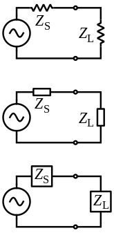
Generalized impedances in a circuit can be drawn with the same symbol as a resistor (US ANSI or DIN Euro) or with a labeled box.

To simplify calculations, sinusoidal voltage and current waves are commonly represented as complex-valued functions of time denoted as V{displaystyle scriptstyle V} and I{displaystyle scriptstyle I}.^[7][8]

V=|V|ej(ωt+ϕV),I=|I|ej(ωt+ϕI).{displaystyle {begin{aligned}V&=|V|e^{j(omega t+phi _{V})},\I&=|I|e^{j(omega t+phi _{I})}.end{aligned}}}

The impedance of a bipolar circuit is defined as the ratio of these quantities:

Z=VI=|V||I|ej(ϕV−ϕI).{displaystyle Z={frac {V}{I}}={frac {|V|}{|I|}}e^{j(phi _{V}-phi _{I})}.}

Hence, denoting θ=ϕV−ϕI{displaystyle theta =phi _{V}-phi _{I}}, we have

|V|=|I||Z|,ϕV=ϕI+θ.{displaystyle {begin{aligned}|V|&=|I||Z|,\phi _{V}&=phi _{I}+theta .end{aligned}}}

The magnitude equation is the familiar Ohm's law applied to the voltage and current amplitudes, while the second equation defines the phase relationship.

Validity of complex representation

This representation using complex exponentials may be justified by noting that (by Euler's formula):

 cos⁡(ωt+ϕ)=12[ej(ωt+ϕ)+e−j(ωt+ϕ)]{displaystyle cos(omega t+phi )={frac {1}{2}}{Big [}e^{j(omega t+phi )}+e^{-j(omega t+phi )}{Big ]}}

The real-valued sinusoidal function representing either voltage or current may be broken into two complex-valued functions. By the principle of superposition, we may analyse the behaviour of the sinusoid on the left-hand side by analysing the behaviour of the two complex terms on the right-hand side. Given the symmetry, we only need to perform the analysis for one right-hand term. The results are identical for the other. At the end of any calculation, we may return to real-valued sinusoids by further noting that

 cos⁡(ωt+ϕ)=ℜ{ej(ωt+ϕ)}{displaystyle cos(omega t+phi )=Re {Big {}e^{j(omega t+phi )}{Big }}}

Ohm's law

An AC supply applying a voltage V{displaystyle scriptstyle V}, across a load Z{displaystyle scriptstyle Z}, driving a current I{displaystyle scriptstyle I}.

The meaning of electrical impedance can be understood by substituting it into Ohm's law.^[9][10]
Assuming a two-terminal circuit element with impedance Z{displaystyle scriptstyle Z} is driven by a sinusoidal voltage or current as above, there holds

 V=IZ=I|Z|ejarg⁡(Z){displaystyle V=IZ=I|Z|e^{jarg(Z)}}

The magnitude of the impedance |Z|{displaystyle scriptstyle |Z|} acts just like resistance, giving the drop in voltage amplitude across an impedance Z{displaystyle scriptstyle Z} for a given current I{displaystyle scriptstyle I}. The phase factor tells us that the current lags the voltage by a phase of θ=arg⁡(Z){displaystyle scriptstyle theta ;=;arg(Z)} (i.e., in the time domain, the current signal is shifted θ2πT{displaystyle scriptstyle {frac {theta }{2pi }}T} later with respect to the voltage signal).

Just as impedance extends Ohm's law to cover AC circuits, other results from DC circuit analysis, such as voltage division, current division, Thévenin's theorem and Norton's theorem, can also be extended to AC circuits by replacing resistance with impedance.

Phasors

A phasor is represented by a constant complex number, usually expressed in exponential form, representing the complex amplitude (magnitude and phase) of a sinusoidal function of time. Phasors are used by electrical engineers to simplify computations involving sinusoids, where they can often reduce a differential equation problem to an algebraic one.

The impedance of a circuit element can be defined as the ratio of the phasor voltage across the element to the phasor current through the element, as determined by the relative amplitudes and phases of the voltage and current. This is identical to the definition from Ohm's law given above, recognising that the factors of ejωt{displaystyle scriptstyle e^{jomega t}} cancel.

Device examples

Resistor

The phase angles in the equations for the impedance of capacitors and inductors indicate that the voltage across a capacitor lags the current through it by a phase of π/2{displaystyle pi /2}, while the voltage across an inductor leads the current through it by π/2{displaystyle pi /2}. The identical voltage and current amplitudes indicate that the magnitude of the impedance is equal to one.

The impedance of an ideal resistor is purely real and is called resistive impedance:

 ZR=R{displaystyle Z_{R}=R}

In this case, the voltage and current waveforms are proportional and in phase.

Inductor and capacitor

Ideal inductors and capacitors have a purely imaginary reactive impedance:

the impedance of inductors increases as frequency increases;

 ZL=jωL{displaystyle Z_{L}=jomega L}

the impedance of capacitors decreases as frequency increases;

 ZC=1jωC{displaystyle Z_{C}={frac {1}{jomega C}}}

In both cases, for an applied sinusoidal voltage, the resulting current is also sinusoidal, but in quadrature, 90 degrees out of phase with the voltage. However, the phases have opposite signs: in an inductor, the current is lagging; in a capacitor the current is leading.

Note the following identities for the imaginary unit and its reciprocal:

j≡cos⁡(π2)+jsin⁡(π2)≡ejπ21j≡−j≡cos⁡(−π2)+jsin⁡(−π2)≡ej(−π2){displaystyle {begin{aligned}j&equiv cos {left({frac {pi }{2}}right)}+jsin {left({frac {pi }{2}}right)}equiv e^{j{frac {pi }{2}}}\{frac {1}{j}}equiv -j&equiv cos {left(-{frac {pi }{2}}right)}+jsin {left(-{frac {pi }{2}}right)}equiv e^{j(-{frac {pi }{2}})}end{aligned}}}

Thus the inductor and capacitor impedance equations can be rewritten in polar form:

ZL=ωLejπ2ZC=1ωCej(−π2){displaystyle {begin{aligned}Z_{L}&=omega Le^{j{frac {pi }{2}}}\Z_{C}&={frac {1}{omega C}}e^{jleft(-{frac {pi }{2}}right)}end{aligned}}}

The magnitude gives the change in voltage amplitude for a given current amplitude through the impedance, while the exponential factors give the phase relationship.

Deriving the device-specific impedances

What follows below is a derivation of impedance for each of the three basic circuit elements: the resistor, the capacitor, and the inductor. Although the idea can be extended to define the relationship between the voltage and current of any arbitrary signal, these derivations assume sinusoidal signals. In fact, this applies to any arbitrary periodic signals, because these can be approximated as a sum of sinusoids through Fourier analysis.

Resistor

For a resistor, there is the relation

vR(t)=iR(t)R{displaystyle v_{text{R}}left(tright)={i_{text{R}}left(tright)}R}

which is Ohm's law.

Considering the voltage signal to be

vR(t)=Vpsin⁡(ωt){displaystyle v_{text{R}}(t)=V_{p}sin(omega t)}

it follows that

vR(t)iR(t)=Vpsin⁡(ωt)Ipsin⁡(ωt)=R{displaystyle {frac {v_{text{R}}left(tright)}{i_{text{R}}left(tright)}}={frac {V_{p}sin(omega t)}{I_{p}sin left(omega tright)}}=R}

This says that the ratio of AC voltage amplitude to alternating current (AC) amplitude across a resistor is R{displaystyle scriptstyle R}, and that the AC voltage leads the current across a resistor by 0 degrees.

This result is commonly expressed as

Zresistor=R{displaystyle Z_{text{resistor}}=R}

Capacitor

For a capacitor, there is the relation:

iC(t)=Cd⁡vC(t)d⁡t{displaystyle i_{text{C}}(t)=C{frac {operatorname {d} v_{text{C}}(t)}{operatorname {d} t}}}

Considering the voltage signal to be

vC(t)=Vpejωt{displaystyle v_{text{C}}(t)=V_{p}e^{jomega t},}

it follows that

d⁡vC(t)d⁡t=jωVpejωt{displaystyle {frac {operatorname {d} v_{text{C}}(t)}{operatorname {d} t}}=jomega V_{p}e^{jomega t}}

and thus, as previously,

Zcapacitor=vC(t)iC(t)=1jωC.{displaystyle Z_{text{capacitor}}={frac {v_{text{C}}left(tright)}{i_{text{C}}left(tright)}}={1 over jomega C}.}

Conversely, if the current through the circuit is assumed to be sinusoidal, its complex representation being

iC(t)=Ipejωt{displaystyle i_{text{C}}(t)=I_{p}e^{jomega t},}

then integrating the differential equation

iC(t)=Cd⁡vC(t)d⁡t{displaystyle i_{text{C}}(t)=C{frac {operatorname {d} v_{text{C}}(t)}{operatorname {d} t}}}

leads to

vC(t)=1jωCIpejωt+Const=1jωCiC(t)+Const.{displaystyle v_{C}(t)={1 over jomega C}I_{p}e^{jomega t}+{text{Const}}={1 over jomega C}i_{C}(t)+{text{Const}}.}

The Const term represents a fixed potential bias superimposed to the AC sinusoidal potential, that plays no role in AC analysis. For this purpose, this term can be assumed to be 0, hence again the impedance

Zcapacitor=1jωC.{displaystyle Z_{text{capacitor}}={1 over jomega C}.}

Inductor

For the inductor, we have the relation (from Faraday's law):

vL(t)=Ld⁡iL(t)d⁡t{displaystyle v_{text{L}}(t)=L{frac {operatorname {d} i_{text{L}}(t)}{operatorname {d} t}}}

This time, considering the current signal to be:

iL(t)=Ipsin⁡(ωt){displaystyle i_{text{L}}(t)=I_{p}sin(omega t)}

it follows that:

d⁡iL(t)d⁡t=ωIpcos⁡(ωt){displaystyle {frac {operatorname {d} i_{text{L}}(t)}{operatorname {d} t}}=omega I_{p}cos left(omega tright)}

This result is commonly expressed in polar form as

 Zinductor=ωLejπ2{displaystyle Z_{text{inductor}}=omega Le^{j{frac {pi }{2}}}}

or, using Euler's formula, as

 Zinductor=jωL{displaystyle Z_{text{inductor}}=jomega L}

As in the case of capacitors, it is also possible to derive this formula directly from the complex representations of the voltages and currents, or by assuming a sinusoidal voltage between the two poles of the inductor.
In this later case, integrating the differential equation above leads to a Const term for the current, that represents a fixed DC bias flowing through the inductor. This is set to zero because AC analysis using frequency domain impedance considers one frequency at a time and DC represents a separate frequency of zero hertz in this context.

Generalised s-plane impedance

Impedance defined in terms of jω can strictly be applied only to circuits that are driven with a steady-state AC signal. The concept of impedance can be extended to a circuit energised with any arbitrary signal by using complex frequency instead of jω. Complex frequency is given the symbol s and is, in general, a complex number. Signals are expressed in terms of complex frequency by taking the Laplace transform of the time domain expression of the signal. The impedance of the basic circuit elements in this more general notation is as follows:

Element	Impedance expression
Resistor	R{displaystyle R,}
Inductor	sL{displaystyle sL,}
Capacitor	1sC{displaystyle {frac {1}{sC}},}

For a DC circuit, this simplifies to s = 0. For a steady-state sinusoidal AC signal s = jω.

Resistance vs reactance

Resistance and reactance together determine the magnitude and phase of the impedance through the following relations:

|Z|=ZZ∗=R2+X2θ=arctan⁡(XR){displaystyle {begin{aligned}|Z|&={sqrt {ZZ^{*}}}={sqrt {R^{2}+X^{2}}}\theta &=arctan {left({frac {X}{R}}right)}end{aligned}}}

In many applications, the relative phase of the voltage and current is not critical so only the magnitude of the impedance is significant.

Resistance

Resistance R{displaystyle R} is the real part of impedance; a device with a purely resistive impedance exhibits no phase shift between the voltage and current.

 R=|Z|cos⁡θ{displaystyle R=|Z|cos {theta }quad }

Reactance

Reactance X{displaystyle X} is the imaginary part of the impedance; a component with a finite reactance induces a phase shift θ{displaystyle theta } between the voltage across it and the current through it.

 X=|Z|sin⁡θ{displaystyle X=|Z|sin {theta }quad }

A purely reactive component is distinguished by the sinusoidal voltage across the component being in quadrature with the sinusoidal current through the component. This implies that the component alternately absorbs energy from the circuit and then returns energy to the circuit. A pure reactance does not dissipate any power.

Capacitive reactance

A capacitor has a purely reactive impedance that is inversely proportional to the signal frequency. A capacitor consists of two conductors separated by an insulator, also known as a dielectric.

XC=−(ωC)−1=−(2πfC)−1{displaystyle X_{C}=-(omega C)^{-1}=-(2pi fC)^{-1}quad }

The minus sign indicates that the imaginary part of the impedance is negative.

At low frequencies, a capacitor approaches an open circuit so no current flows through it.

A DC voltage applied across a capacitor causes charge to accumulate on one side; the electric field due to the accumulated charge is the source of the opposition to the current. When the potential associated with the charge exactly balances the applied voltage, the current goes to zero.

Driven by an AC supply, a capacitor accumulates only a limited charge before the potential difference changes sign and the charge dissipates. The higher the frequency, the less charge accumulates and the smaller the opposition to the current.

Inductive reactance

Inductive reactance XL{displaystyle X_{L}} is proportional to the signal frequency f{displaystyle f} and the inductance L{displaystyle L}.

XL=ωL=2πfL{displaystyle X_{L}=omega L=2pi fLquad }

An inductor consists of a coiled conductor. Faraday's law of electromagnetic induction gives the back emf E{displaystyle {mathcal {E}}} (voltage opposing current) due to a rate-of-change of magnetic flux density B{displaystyle B} through a current loop.

E=−dΦBdt{displaystyle {mathcal {E}}=-{{dPhi _{B}} over dt}quad }

For an inductor consisting of a coil with N{displaystyle N} loops this gives:

E=−NdΦBdt{displaystyle {mathcal {E}}=-N{dPhi _{B} over dt}quad }

The back-emf is the source of the opposition to current flow. A constant direct current has a zero rate-of-change, and sees an inductor as a short-circuit (it is typically made from a material with a low resistivity). An alternating current has a time-averaged rate-of-change that is proportional to frequency, this causes the increase in inductive reactance with frequency.

Total reactance

The total reactance is given by

X=XL+XC{displaystyle {X=X_{L}+X_{C}}} (note that XC{displaystyle X_{C}} is negative)

so that the total impedance is

 Z=R+jX{displaystyle Z=R+jX}

Combining impedances

The total impedance of many simple networks of components can be calculated using the rules for combining impedances in series and parallel. The rules are identical to those for combining resistances, except that the numbers in general are complex numbers. The general case, however, requires equivalent impedance transforms in addition to series and parallel.

Series combination

For components connected in series, the current through each circuit element is the same; the total impedance is the sum of the component impedances.

 Zeq=Z1+Z2+⋯+Zn{displaystyle Z_{text{eq}}=Z_{1}+Z_{2}+cdots +Z_{n}quad }

Or explicitly in real and imaginary terms:

 Zeq=R+jX=(R1+R2+⋯+Rn)+j(X1+X2+⋯+Xn){displaystyle Z_{text{eq}}=R+jX=(R_{1}+R_{2}+cdots +R_{n})+j(X_{1}+X_{2}+cdots +X_{n})quad }

Parallel combination

For components connected in parallel, the voltage across each circuit element is the same; the ratio of currents through any two elements is the inverse ratio of their impedances.

Hence the inverse total impedance is the sum of the inverses of the component impedances:

1Zeq=1Z1+1Z2+⋯+1Zn{displaystyle {frac {1}{Z_{text{eq}}}}={frac {1}{Z_{1}}}+{frac {1}{Z_{2}}}+cdots +{frac {1}{Z_{n}}}}

or, when n = 2:

1Zeq=1Z1+1Z2=Z1+Z2Z1Z2{displaystyle {frac {1}{Z_{text{eq}}}}={frac {1}{Z_{1}}}+{frac {1}{Z_{2}}}={frac {Z_{1}+Z_{2}}{Z_{1}Z_{2}}}}

 Zeq=Z1Z2Z1+Z2{displaystyle Z_{text{eq}}={frac {Z_{1}Z_{2}}{Z_{1}+Z_{2}}}}

The equivalent impedance Zeq{displaystyle scriptstyle Z_{text{eq}}} can be calculated in terms of the equivalent series resistance Req{displaystyle scriptstyle R_{text{eq}}} and reactance Xeq{displaystyle scriptstyle X_{text{eq}}}.^[11]

Zeq=Req+jXeqReq=(X1R2+X2R1)(X1+X2)+(R1R2−X1X2)(R1+R2)(R1+R2)2+(X1+X2)2Xeq=(X1R2+X2R1)(R1+R2)−(R1R2−X1X2)(X1+X2)(R1+R2)2+(X1+X2)2{displaystyle {begin{aligned}Z_{text{eq}}&=R_{text{eq}}+jX_{text{eq}}\R_{text{eq}}&={frac {(X_{1}R_{2}+X_{2}R_{1})(X_{1}+X_{2})+(R_{1}R_{2}-X_{1}X_{2})(R_{1}+R_{2})}{(R_{1}+R_{2})^{2}+(X_{1}+X_{2})^{2}}}\X_{text{eq}}&={frac {(X_{1}R_{2}+X_{2}R_{1})(R_{1}+R_{2})-(R_{1}R_{2}-X_{1}X_{2})(X_{1}+X_{2})}{(R_{1}+R_{2})^{2}+(X_{1}+X_{2})^{2}}}end{aligned}}}

Measurement

The measurement of the impedance of devices and transmission lines is a practical problem in radio technology and other fields. Measurements of impedance may be carried out at one frequency, or the variation of device impedance over a range of frequencies may be of interest. The impedance may be measured or displayed directly in ohms, or other values related to impedance may be displayed; for example, in a radio antenna, the standing wave ratio or reflection coefficient may be more useful than the impedance alone. The measurement of impedance requires the measurement of the magnitude of voltage and current, and the phase difference between them. Impedance is often measured by "bridge" methods, similar to the direct-current Wheatstone bridge; a calibrated reference impedance is adjusted to balance off the effect of the impedance of the device under test. Impedance measurement in power electronic devices may require simultaneous measurement and provision of power to the operating device.

The impedance of a device can be calculated by complex division of the voltage and current. The impedance of the device can be calculated by applying a sinusoidal voltage to the device in series with a resistor, and measuring the voltage across the resistor and across the device. Performing this measurement by sweeping the frequencies of the applied signal provides the impedance phase and magnitude.^[12]

The use of an impulse response may be used in combination with the fast Fourier transform (FFT) to rapidly measure the electrical impedance of various electrical devices.^[12]

The LCR meter (Inductance (L), Capacitance (C), and Resistance (R)) is a device commonly used to measure the inductance, resistance and capacitance of a component; from these values, the impedance at any frequency can be calculated.

Example

Consider an LC tank circuit.
The complex impedance of the circuit is

Z(ω)=jωL1−ω2LC.{displaystyle Z(omega )={jomega L over 1-omega ^{2}LC}.}

It is immediately seen that the value of 1|Z|{displaystyle {1 over |Z|}} is minimal (actually equal to 0 in this case) whenever

ω2LC=1.{displaystyle omega ^{2}LC=1.}

Therefore, the fundamental resonance angular frequency is

ω=1LC.{displaystyle omega ={1 over {sqrt {LC}}}.}

Variable impedance

In general, neither impedance nor admittance can vary with time, since they are defined for complex exponentials in which −∞ < t < +∞ . If the complex exponential voltage to current ratio changes over time or amplitude, the circuit element cannot be described using the frequency domain. However, many systems (e.g., varicaps that are used in radio tuners) may exhibit non-linear or time-varying voltage to current ratios that seem to be linear time-invariant (LTI) for small signals and over small observation windows, so they can be roughly described as-if they had a time-varying impedance. This description is an approximation: Over large signal swings or wide observation windows, the voltage to current relationship will not be LTI and cannot be described by impedance.

See also

• Bioelectrical impedance analysis


• Characteristic impedance


• Electrical characteristics of dynamic loudspeakers


• High impedance


• Immittance


• Impedance bridging


• Impedance cardiography


• Impedance control


• Impedance matching


• Impedance microbiology


• Negative impedance converter


• Resistance distance

References

External links

• Explaining Impedance


• Antenna Impedance


• 
  ECE 209: Review of Circuits as LTI Systems – Brief explanation of Laplace-domain circuit analysis; includes a definition of impedance.

References

^ Callegaro, p. 2
^ Callegaro, Sec. 1.6
^ Science, p. 18, 1888
^ Oliver Heaviside, The Electrician, p. 212, 23 July 1886, reprinted as Electrical Papers, p 64, AMS Bookstore, .mw-parser-output cite.citation{font-style:inherit}.mw-parser-output q{quotes:"""""""'""'"}.mw-parser-output code.cs1-code{color:inherit;background:inherit;border:inherit;padding:inherit}.mw-parser-output .cs1-lock-free a{background:url("//upload.wikimedia.org/wikipedia/commons/thumb/6/65/Lock-green.svg/9px-Lock-green.svg.png")no-repeat;background-position:right .1em center}.mw-parser-output .cs1-lock-limited a,.mw-parser-output .cs1-lock-registration a{background:url("//upload.wikimedia.org/wikipedia/commons/thumb/d/d6/Lock-gray-alt-2.svg/9px-Lock-gray-alt-2.svg.png")no-repeat;background-position:right .1em center}.mw-parser-output .cs1-lock-subscription a{background:url("//upload.wikimedia.org/wikipedia/commons/thumb/a/aa/Lock-red-alt-2.svg/9px-Lock-red-alt-2.svg.png")no-repeat;background-position:right .1em center}.mw-parser-output .cs1-subscription,.mw-parser-output .cs1-registration{color:#555}.mw-parser-output .cs1-subscription span,.mw-parser-output .cs1-registration span{border-bottom:1px dotted;cursor:help}.mw-parser-output .cs1-hidden-error{display:none;font-size:100%}.mw-parser-output .cs1-visible-error{font-size:100%}.mw-parser-output .cs1-subscription,.mw-parser-output .cs1-registration,.mw-parser-output .cs1-format{font-size:95%}.mw-parser-output .cs1-kern-left,.mw-parser-output .cs1-kern-wl-left{padding-left:0.2em}.mw-parser-output .cs1-kern-right,.mw-parser-output .cs1-kern-wl-right{padding-right:0.2em}
ISBN 0-8218-3465-7
^ Kennelly, Arthur. Impedance (AIEE, 1893)
^ Alexander, Charles; Sadiku, Matthew (2006). Fundamentals of Electric Circuits (3, revised ed.). McGraw-Hill. pp. 387–389. ISBN 978-0-07-330115-0
^ Complex impedance, Hyperphysics
^ Horowitz, Paul; Hill, Winfield (1989). "1". The Art of Electronics. Cambridge University Press. pp. 31–32. ISBN 0-521-37095-7.
^ AC Ohm's law, Hyperphysics
^ Horowitz, Paul; Hill, Winfield (1989). "1". The Art of Electronics. Cambridge University Press. pp. 32–33. ISBN 0-521-37095-7.
^ Parallel Impedance Expressions, Hyperphysics
^ ab George Lewis Jr.; George K. Lewis Sr. & William Olbricht (August 2008). "Cost-effective broad-band electrical impedance spectroscopy measurement circuit and signal analysis for piezo-materials and ultrasound transducers". Measurement Science and Technology. 19 (10): 105102. Bibcode:2008MeScT..19j5102L. doi:10.1088/0957-0233/19/10/105102. PMC 2600501. PMID 19081773. Retrieved 2008-09-15.