Agfdhyk

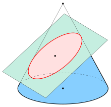
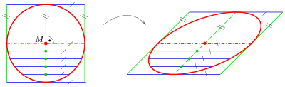
An ellipse (red) obtained as the intersection of a cone with an inclined plane

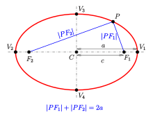
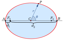
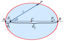
Ellipse: notations

Ellipses: examples

In mathematics, an ellipse is a curve in a plane surrounding two focal points such that the sum of the distances to the two focal points is constant for every point on the curve. As such, it is a generalization of a circle, which is a special type of an ellipse having both focal points at the same location. The elongation of an ellipse is represented by its eccentricity, which for an ellipse can be any number from 0 (the limiting case of a circle) to arbitrarily close to but less than 1.

Ellipses are the closed type of conic section: a plane curve resulting from the intersection of a cone by a plane (see figure to the right). Ellipses have many similarities with the other two forms of conic sections: parabolas and hyperbolas, both of which are open and unbounded. The cross section of a cylinder is an ellipse, unless the section is parallel to the axis of the cylinder.

Analytically, an ellipse may also be defined as the set of points such that the ratio of the distance of each point on the curve from a given point (called a focus or focal point) to the distance from that same point on the curve to a given line (called the directrix) is a constant. This ratio is the above-mentioned eccentricity of the ellipse.

An ellipse may also be defined analytically as the set of points for each of which the sum of its distances to two foci is a fixed number.

Ellipses are common in physics, astronomy and engineering. For example, the orbit of each planet in the solar system is approximately an ellipse with the barycenter of the planet–Sun pair at one of the focal points. The same is true for moons orbiting planets and all other systems having two astronomical bodies. The shapes of planets and stars are often well described by ellipsoids. Ellipses also arise as images of a circle under parallel projection and the bounded cases of perspective projection, which are simply intersections of the projective cone with the plane of projection. It is also the simplest Lissajous figure formed when the horizontal and vertical motions are sinusoids with the same frequency. A similar effect leads to elliptical polarization of light in optics.

The name, ἔλλειψις (élleipsis, "omission"), was given by Apollonius of Perga in his Conics, emphasizing the connection of the curve with "application of areas".

Definition of an ellipse as locus of points

Ellipse: Definition

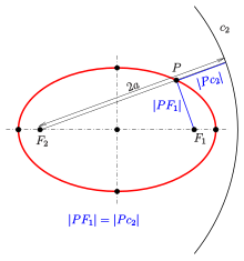
Ellipse: definition with director circle

An ellipse can be defined geometrically as a set of points (locus of points) in the Euclidean plane:

• An ellipse can be defined using two fixed points, F1{displaystyle F_{1}}, F2{displaystyle F_{2}}, called the foci and a distance, usually denoted 2a{displaystyle 2a}. The ellipse defined with F1{displaystyle F_{1}}, F2{displaystyle F_{2}} and 2a{displaystyle 2a} is the set of points P{displaystyle P} such that the sum of the distances |PF1|, |PF2|{displaystyle |PF_{1}|, |PF_{2}|} is constant and equal to 2a{displaystyle 2a}. In order to omit the special case of a line segment, one assumes 2a>|F1F2|.{displaystyle 2a>|F_{1}F_{2}|.} More formally, for a given a{displaystyle a}, an ellipse is the set E={P∈R2∣|PF2|+|PF1|=2a} .{displaystyle E={Pin mathbb {R} ^{2}mid |PF_{2}|+|PF_{1}|=2a} .}
  

The midpoint C{displaystyle C} of the line segment joining the foci is called the center of the ellipse. The line through the foci is called the major axis, and the line perpendicular to it through the center is called the minor axis. The major axis contains the vertices V1,V2{displaystyle V_{1},V_{2}}, which have distance a{displaystyle a} to the center. The distance c{displaystyle c} of the foci to the center is called the focal distance or linear eccentricity. The quotient ca{displaystyle {tfrac {c}{a}}} is the eccentricity e{displaystyle e}.

The case F1=F2{displaystyle F_{1}=F_{2}} yields a circle and is included.

The equation |PF2|+|PF1|=2a{displaystyle |PF_{2}|+|PF_{1}|=2a} can be viewed in a different way (see picture):

If c2{displaystyle c_{2}} is the circle with midpoint F2{displaystyle F_{2}} and radius 2a{displaystyle 2a}, then the distance of a point P{displaystyle P} to the circle c2{displaystyle c_{2}} equals the distance to the focus F1{displaystyle F_{1}}:

|PF1|=|Pc2|.{displaystyle |PF_{1}|=|Pc_{2}|.}

c2{displaystyle c_{2}} is called the circular directrix (related to focus F2{displaystyle F_{2}}) of the ellipse.^[1][2] This property should not be confused with the definition of an ellipse with help of a directrix (line) below.

Using Dandelin spheres one can prove that any plane section of a cone with a plane, which does not contain the apex and whose slope is less than the slope of the lines on the cone, is an ellipse.

Ellipse in Cartesian coordinates

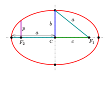
shape parameters:
a: semi-major axis,
b: semi-minor axis
c: linear eccentricity,
p: semi-latus rectum.

Equation

If Cartesian coordinates are introduced such that the origin is the center of the ellipse and the x-axis is the major axis and

the foci are the points F1=(c,0), F2=(−c,0){displaystyle F_{1}=(c,0), F_{2}=(-c,0)},

the vertices are V1=(a,0), V2=(−a,0){displaystyle V_{1}=(a,0), V_{2}=(-a,0)}.

For an arbitrary point (x,y){displaystyle (x,y)} the distance to the focus (c,0){displaystyle (c,0)} is
(x−c)2+y2{displaystyle {sqrt {(x-c)^{2}+y^{2}}}} and to the second focus (x+c)2+y2{displaystyle {sqrt {(x+c)^{2}+y^{2}}}}. Hence the point (x,y){displaystyle (x,y)} is on the ellipse if the following condition is fulfilled

(x−c)2+y2+(x+c)2+y2=2a .{displaystyle {sqrt {(x-c)^{2}+y^{2}}}+{sqrt {(x+c)^{2}+y^{2}}}=2a .}

Remove the square roots by suitable squarings and use the relation b2=a2−c2{displaystyle b^{2}=a^{2}-c^{2}} to obtain the equation of the ellipse:

• x2a2+y2b2=1,{displaystyle {frac {x^{2}}{a^{2}}}+{frac {y^{2}}{b^{2}}}=1,}

or, solved for y,

y=±baa2−x2.{displaystyle y=pm {frac {b}{a}}{sqrt {a^{2}-x^{2}}}.}

The shape parameters a,b{displaystyle a,;b} are called the semi-major and semi-minor axes. The points V3=(0,b),V4=(0,−b){displaystyle V_{3}=(0,b),;V_{4}=(0,-b)} are the co-vertices.

It follows from the equation that the ellipse is symmetric with respect to both of the coordinate axes and hence symmetric with respect to the origin.

Eccentricity

The eccentricity of an ellipse can be expressed in terms of the ratio of semi-minor and semi-major axes as

e=1−(ba)2.{displaystyle e={sqrt {1-left({frac {b}{a}}right)^{2}}}.}

This definition relies on the major axis 2a of an ellipse not being shorter than its minor axis 2b. Ellipses with equal axes are simply circles, that is, ellipses with zero eccentricity. The degree of flatness of ellipses increases as their eccentricity does.

Semi-latus rectum

The length of the chord through one of the foci, which is perpendicular to the major axis of the ellipse is called the latus rectum. One half of it is the semi-latus rectum p{displaystyle p}. A calculation shows

• p=b2a.{displaystyle p={frac {b^{2}}{a}}.}

The semi-latus rectum p{displaystyle p} may also be viewed as the radius of curvature of the osculating circles at the vertices on the major axis.

Tangent

An arbitrary line g{displaystyle g} intersects an ellipse at 0, 1 or 2 points. In the first case the line is called exterior line, in the second case tangent and secant in the third case. Through any point of an ellipse there is exactly one tangent.

The tangent at a point (x0,y0){displaystyle (x_{0},y_{0})} of the ellipse x2a2+y2b2=1{displaystyle ;{tfrac {x^{2}}{a^{2}}}+{tfrac {y^{2}}{b^{2}}}=1;} has the coordinate equation

•  x0a2x+y0b2y=1.{displaystyle {frac {x_{0}}{a^{2}}}x+{frac {y_{0}}{b^{2}}}y=1;.}

A vector equation of the tangent is

• 
   x→=(x0y0)+s(−y0a2x0b2){displaystyle {vec {x}}={begin{pmatrix}x_{0}\y_{0}end{pmatrix}}+s;{begin{pmatrix}-y_{0}a^{2}\x_{0}b^{2}end{pmatrix}}quad } withs∈R .{displaystyle quad sin mathbb {R} .}
  

Proof:
Let be (x0,y0){displaystyle (x_{0},y_{0})} an ellipse point and x→=(x0y0)+s(uv){displaystyle ;{vec {x}}={begin{pmatrix}x_{0}\y_{0}end{pmatrix}}+s;{begin{pmatrix}u\vend{pmatrix}};} the vector equation of a line g{displaystyle g} (containing (x0,y0){displaystyle (x_{0},y_{0})}). Inserting the line's equation into the ellipse equation and respecting x02a2+y02b2=1{displaystyle ;{tfrac {x_{0}^{2}}{a^{2}}}+{tfrac {y_{0}^{2}}{b^{2}}}=1;} yields:

(x0+su)2a2+(y0+sv)2b2=1 ,⟶2s(x0ua2+y0vb2)+s2(u2a2+v2b2)=0 .{displaystyle {frac {(x_{0}+su)^{2}}{a^{2}}}+{frac {(y_{0}+sv)^{2}}{b^{2}}}=1 ,quad longrightarrow quad 2s;left({frac {x_{0}u}{a^{2}}}+{frac {y_{0}v}{b^{2}}}right)+s^{2};left({frac {u^{2}}{a^{2}}}+{frac {v^{2}}{b^{2}}}right)=0 .}

In case of (1)x0a2u+y0b2v=0{displaystyle ;(1);{tfrac {x_{0}}{a^{2}}}u+{tfrac {y_{0}}{b^{2}}}v=0;} line g{displaystyle g} and the ellipse have only point (x0,y0){displaystyle (x_{0},y_{0})} in common and g{displaystyle g} is a tangent. The tangent direction is orthogonal to vector (x0a2,y0b2)T{displaystyle ({tfrac {x_{0}}{a^{2}}},{tfrac {y_{0}}{b^{2}}})^{T}} which is then a normal vector of the tangent and the tangent has the equation x0a2x+y0b2y=k{displaystyle ;{tfrac {x_{0}}{a^{2}}}x+{tfrac {y_{0}}{b^{2}}}y=k;} with a still unknown k{displaystyle k}. Because (x0,y0){displaystyle (x_{0},y_{0})} is on the tangent and on the ellipse, one gets k=1{displaystyle k=1}.

In case of (2)x0a2u+y0b2v≠0{displaystyle ;(2);{tfrac {x_{0}}{a^{2}}}u+{tfrac {y_{0}}{b^{2}}}vneq 0;} line g{displaystyle g} has a second point with the ellipse in common.

With help of (1) one finds that (−y0a2,x0b2)T{displaystyle ;(-y_{0}a^{2},x_{0}b^{2})^{T};} is a tangent vector at point (x0,y0){displaystyle (x_{0},y_{0})}, which proves the vector equation.

If (x0,y0){displaystyle (x_{0},y_{0})} and (u,v){displaystyle (u,v)} are two points of the ellipse, such that
x0ua2+y0vb2=0{displaystyle ;{tfrac {x_{0}u}{a^{2}}}+{tfrac {y_{0}v}{b^{2}}}=0;} holds, then the points lie on two conjugate diameters of the Ellipse (see below). In case of a=b{displaystyle a=b} the ellipse is a circle and "conjugate" means "orthogonal".

Equation of a shifted ellipse

If the ellipse is shifted such that its center is (c1,c2){displaystyle (c_{1},c_{2})} the equation is

• (x−c1)2a2+(y−c2)2b2=1 .{displaystyle {frac {(x-c_{1})^{2}}{a^{2}}}+{frac {(y-c_{2})^{2}}{b^{2}}}=1 .}

The axes are still parallel to the x- and y-axes.

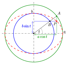
The construction of points based on the parametric equation and the interpretation of parameter t, which is due to de la Hire

Parametric representation

Ellipse points calculated by the rational representation with equal spaced parameters (Δu=0.2{displaystyle Delta u=0.2})

Standard parametric representation

Using the sine and cosine functions cos,sin{displaystyle cos ,sin }, a parametric representation of the ellipse x2a2+y2b2=1{displaystyle {tfrac {x^{2}}{a^{2}}}+{tfrac {y^{2}}{b^{2}}}=1} can be obtained, :

• (x,y)=(acos⁡t,bsin⁡t), 0≤t<2π .{displaystyle (x,y)=(acos t,bsin t), 0leq t<2pi .}

Parameter t can be taken as shown in the diagram and is due to de la Hire.^[3]

The parameter t (called the eccentric anomaly in astronomy) is not the angle of (x(t),y(t))T{displaystyle (x(t),y(t))^{T}} with the x-axis (see diagram at right). For other interpretations of parameter t see section Drawing ellipses.

Rational representation

With the substitution u=tan⁡(t/2){displaystyle u=tan(t/2)} and trigonometric formulae one gets

cos⁡t=(1−u2)/(u2+1) ,sin⁡t=2u/(u2+1){displaystyle cos t=(1-u^{2})/(u^{2}+1) ,quad sin t=2u/(u^{2}+1)}

and the rational parametric equation of an ellipse

•  x(u)=a(1−u2)/(u2+1)y(u)=2bu/(u2+1),−∞<u<∞,{displaystyle {begin{array}{lcl}x(u)&=&a(1-u^{2})/(u^{2}+1)\y(u)&=&2bu/(u^{2}+1)end{array}};,quad -infty <u<infty ;,}

which covers any point of the ellipse x2a2+y2b2=1{displaystyle ;{tfrac {x^{2}}{a^{2}}}+{tfrac {y^{2}}{b^{2}}}=1;} except the left vertex (−a,0){displaystyle (-a,0)}.

For u∈[0,1],{displaystyle uin [0,1],} this formula represents the right upper quarter of the ellipse moving counter-clockwise with increasing u.{displaystyle u.} The left vertex is the limit limu→±∞(x(u),y(u))=(−a,0).{displaystyle lim _{uto pm infty }(x(u),y(u))=(-a,0);.}

Rational representations of conic sections are popular with Computer Aided Design (see Bezier curve).

Tangent slope as parameter

A parametric representation, which uses the slope m{displaystyle m} of the tangent at a point of the ellipse
can be obtained from the derivative of the standard representation x→(t)=(acos⁡t,bsin⁡t)T{displaystyle {vec {x}}(t)=(acos t,bsin t)^{T}}:

x→′(t)=(−asin⁡t,bcos⁡t)T→m=−bacot⁡t→cot⁡t=−mab.{displaystyle {vec {x}}'(t)=(-asin t,bcos t)^{T}quad rightarrow quad m=-{frac {b}{a}}cot tquad rightarrow quad cot t=-{frac {ma}{b}}.}

With help of trigonometric formulae
one gets:

cos⁡t=cot⁡t±1+cot2⁡t=−ma±m2a2+b2 ,sin⁡t=1±1+cot2⁡t=b±m2a2+b2.{displaystyle cos t={frac {cot t}{pm {sqrt {1+cot ^{2}t}}}}={frac {-ma}{pm {sqrt {m^{2}a^{2}+b^{2}}}}} ,quad quad sin t={frac {1}{pm {sqrt {1+cot ^{2}t}}}}={frac {b}{pm {sqrt {m^{2}a^{2}+b^{2}}}}}.}

Replacing cos⁡t{displaystyle cos t} und sin⁡t{displaystyle sin t} of the standard representation one yields

• c→±(m)=(−ma2±m2a2+b2,b2±m2a2+b2)T,m∈R.{displaystyle {vec {c}}_{pm }(m)=left(-{frac {ma^{2}}{pm {sqrt {m^{2}a^{2}+b^{2}}}}};,;{frac {b^{2}}{pm {sqrt {m^{2}a^{2}+b^{2}}}}}right)^{T},,min mathbb {R} .}

Where m{displaystyle m} is the slope of the tangent at the corresponding ellipse point, c→+{displaystyle {vec {c}}_{+}} is the upper and c→−{displaystyle {vec {c}}_{-}} the lower half of the ellipse. The points with vertical tangents (vertices(±a,0){displaystyle (pm a,0)}) are not covered by the representation.

The equation of the tangent at point c→±(m){displaystyle {vec {c}}_{pm }(m)} has the form y=mx+n{displaystyle y=mx+n}. The still unknown n{displaystyle n} can be determined by inserting the coordinates of the corresponding ellipse point c→±(m){displaystyle {vec {c}}_{pm }(m)}:

• y=mx±m2a2+b2.{displaystyle y=mxpm {sqrt {m^{2}a^{2}+b^{2}}};.}

This description of the tangents of an ellipse is an essential tool for the determination of the orthoptic of an ellipse. The orthoptic article contains another proof, which omits differential calculus and trigonometric formulae.

Shifted Ellipse

A shifted ellipse with center (c1,c2){displaystyle (c_{1},c_{2})} can be described by

• (c1+acos⁡t,c2+bsin⁡t), 0≤t<2π .{displaystyle (c_{1}+acos t;,;c_{2}+bsin t), 0leq t<2pi .}

A parametric representation of an arbitrary ellipse is contained in the section Ellipse as an affine image of the unit circle x² + y² = 1 below.

Parameters a and b

The parameters a{displaystyle a} and b{displaystyle b} represent the lengths of line segments and are therefore non-negative real numbers. Throughout this article a{displaystyle a} is the semi-major axis, i.e., a≥b .{displaystyle ageq b .} In general the canonical ellipse equation x2a2+y2b2=1{displaystyle {tfrac {x^{2}}{a^{2}}}+{tfrac {y^{2}}{b^{2}}}=1} may have a<b{displaystyle a<b} (and hence the ellipse would be taller than it is wide); in this form the semi-major axis would be b{displaystyle b}. This form can be converted to the form assumed in the remainder of this article simply by transposing the variable names x{displaystyle x} and y{displaystyle y} and the parameter names a{displaystyle a} and b.{displaystyle b.}

Definition of an ellipse by the directrix property

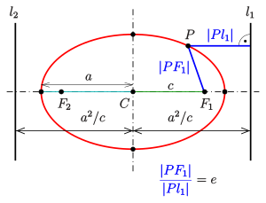
Ellipse: directrix property

The two lines at distance d=a2c{displaystyle d={frac {a^{2}}{c}}} and parallel to the minor axis are called directrices of the ellipse (see diagram).

• For an arbitrary point P{displaystyle P} of the ellipse, the quotient of the distance to one focus and to the corresponding directrix (see diagram) is equal to the eccentricity:

|PF1||Pl1|=|PF2||Pl2|=e=ca .{displaystyle {frac {|PF_{1}|}{|Pl_{1}|}}={frac {|PF_{2}|}{|Pl_{2}|}}=e={frac {c}{a}} .}

The proof for the pair F1,l1{displaystyle F_{1},l_{1}} follows from the fact that |PF1|2=(x−c)2+y2, |Pl1|2=(x−a2c)2{displaystyle |PF_{1}|^{2}=(x-c)^{2}+y^{2}, |Pl_{1}|^{2}=left(x-{tfrac {a^{2}}{c}}right)^{2}} and y2=b2−b2a2x2{displaystyle y^{2}=b^{2}-{tfrac {b^{2}}{a^{2}}}x^{2}} satisfy the equation

|PF1|2−c2a2|Pl1|2=0 .{displaystyle |PF_{1}|^{2}-{frac {c^{2}}{a^{2}}}|Pl_{1}|^{2}=0 .}

The second case is proven analogously.

The inverse statement is also true and can be used to define an ellipse (in a manner similar to the definition of a parabola):

• For any point F{displaystyle F} (focus), any line l{displaystyle l} (directrix) not through F{displaystyle F}, and any real number e{displaystyle e} with 0<e<1,{displaystyle 0<e<1,} the locus of points for which the quotient of the distances to the point and to the line is e,{displaystyle e,} that is,

E={P∣|PF||Pl|=e}{displaystyle E=left{Pmid {frac {|PF|}{|Pl|}}=eright}}

is an ellipse.

The choice e=0{displaystyle e=0}, which is the eccentricity of a circle, is in this context not allowed. One may consider the directrix of a circle to be the line at infinity.

(The choice e=1{displaystyle e=1} yields a parabola, and if e>1{displaystyle e>1}, a hyperbola.)

Pencil of conics with a common vertex and common semi-latus rectum

Proof

Let F=(f,0), e>0{displaystyle F=(f,0), e>0}, and assume (0,0){displaystyle (0,0)} is a point on the curve.
The directrix l{displaystyle l} has equation x=−fe{displaystyle x=-{tfrac {f}{e}}}. With P=(x,y){displaystyle P=(x,y)}, the relation |PF|2=e2|Pl|2{displaystyle |PF|^{2}=e^{2}|Pl|^{2}} produces the equations

(x−f)2+y2=e2(x+fe)2=(ex+f)2{displaystyle (x-f)^{2}+y^{2}=e^{2}left(x+{tfrac {f}{e}}right)^{2}=(ex+f)^{2}} and x2(e2−1)+2xf(1+e)−y2=0.{displaystyle x^{2}(e^{2}-1)+2xf(1+e)-y^{2}=0.}

The substitution p=f(1+e){displaystyle p=f(1+e)} yields

• x2(e2−1)+2px−y2=0.{displaystyle x^{2}(e^{2}-1)+2px-y^{2}=0.}

This is the equation of an ellipse (e<1{displaystyle e<1}), or a parabola (e=1{displaystyle e=1}), or a hyperbola (e>1{displaystyle e>1}). All of these non-degenerate conics have, in common, the origin as a vertex (see diagram).

If e<1{displaystyle e<1}, introduce new parameters a,b{displaystyle a,b} so that
1−e2=b2a2, and  p=b2a{displaystyle 1-e^{2}={tfrac {b^{2}}{a^{2}}},{text{ and }} p={tfrac {b^{2}}{a}}}, and then the equation above becomes

(x−a)2a2+y2b2=1 ,{displaystyle {tfrac {(x-a)^{2}}{a^{2}}}+{tfrac {y^{2}}{b^{2}}}=1 ,}

which is the equation of an ellipse with center (a,0){displaystyle (a,0)}, the x-axis as major axis, and
the major/minor semi axis a,b{displaystyle a,b}.

General case

If the focus is F=(f1,f2){displaystyle F=(f_{1},f_{2})} and the directrix ux+vy+w=0{displaystyle ux+vy+w=0}, one obtains the equation

(x−f1)2+(y−f2)2=e2⋅(ux+vy+w)2u2+v2 .{displaystyle left(x-f_{1}right)^{2}+left(y-f_{2}right)^{2}=e^{2}cdot {frac {left(ux+vy+wright)^{2}}{u^{2}+v^{2}}} .}

(The right side of the equation uses the Hesse normal form of a line to calculate the distance |Pl|{displaystyle |Pl|}.)

The normal bisects the angle between the lines to the foci

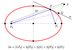
Ellipse: the tangent bisects the supplementary angle of the angle between the lines to the foci.

Rays from one focus reflect off the ellipse to pass through the other focus.

For an ellipse the following statement is true:

• The normal at a point P{displaystyle P} bisects the angle between the lines PF1¯,PF2¯{displaystyle {overline {PF_{1}}},{overline {PF_{2}}}}.

Proof

Because the tangent is perpendicular to the normal, the statement is true for the tangent and the supplementary angle of the angle between the lines to the foci (see diagram), too.

Let L{displaystyle L} be the point on the line PF2¯{displaystyle {overline {PF_{2}}}} with the distance 2a{displaystyle 2a} to the focus F2{displaystyle F_{2}}, a{displaystyle a} is the semi-major axis of the ellipse. Let line w{displaystyle w} be the bisector of the supplementary angle to the angle between the lines PF1¯,PF2¯{displaystyle {overline {PF_{1}}},{overline {PF_{2}}}}. In order to prove that w{displaystyle w} is the tangent line at point P{displaystyle P}, one checks that any point Q{displaystyle Q} on line w{displaystyle w} which is different from P{displaystyle P} cannot be on the ellipse. Hence w{displaystyle w} has only point P{displaystyle P} in common with the ellipse and is, therefore, the tangent at point P{displaystyle P}.

From the diagram and the triangle inequality one recognizes that 2a=|LF2|<|QF2|+|QL|=|QF2|+|QF1|{displaystyle 2a=|LF_{2}|<|QF_{2}|+|QL|=|QF_{2}|+|QF_{1}|} holds, which means: |QF2|+|QF1|>2a{displaystyle |QF_{2}|+|QF_{1}|>2a}. But if Q{displaystyle Q} is a point of the ellipse, the sum should be 2a{displaystyle 2a}.

Application

The rays from one focus are reflected by the ellipse to the second focus. This property has optical and acoustic applications similar to the reflective property of a parabola (see whispering gallery).

Ellipse as an affine image of the unit circle x² + y² = 1

Ellipse as an affine image of the unit circle

Another definition of an ellipse uses affine transformations:

• Any ellipse is the affine image of the unit circle with equation x2+y2=1{displaystyle x^{2}+y^{2}=1}.

An affine transformation of the Euclidean plane has the form x→→f→0+Ax→{displaystyle {vec {x}}to {vec {f}}_{0}+A{vec {x}}}, where A{displaystyle A} is a regular matrix (its determinant is not 0) and f→0{displaystyle {vec {f}}_{0}} is an arbitrary vector. If f→1,f→2{displaystyle {vec {f}}_{1},{vec {f}}_{2}} are the column vectors of the matrix A{displaystyle A}, the unit circle (cos⁡(t),sin⁡(t)),t∈[0,2π),{displaystyle (cos(t),sin(t)),tin [0,2pi ),} is mapped onto the Ellipse

• x→=p→(t)=f→0+f→1cos⁡t+f→2sin⁡t .{displaystyle {vec {x}}={vec {p}}(t)={vec {f}}_{0}+{vec {f}}_{1}cos t+{vec {f}}_{2}sin t .}

f→0{displaystyle {vec {f}}_{0}} is the center, f→1,f→2{displaystyle {vec {f}}_{1},;{vec {f}}_{2}} are the directions of two conjugate diameters of the ellipse. In general the vectors f→1,f→2{displaystyle {vec {f}}_{1},{vec {f}}_{2}} are not perpendicular. That means, in general f→0±f→1{displaystyle {vec {f}}_{0}pm {vec {f}}_{1}} and f→0±f→2{displaystyle {vec {f}}_{0}pm {vec {f}}_{2}} are not the vertices of the ellipse.

The tangent vector at point p→(t){displaystyle {vec {p}}(t)} is

p→′(t)=−f→1sin⁡t+f→2cos⁡t .{displaystyle {vec {p}}'(t)=-{vec {f}}_{1}sin t+{vec {f}}_{2}cos t .}

Because at a vertex the tangent is perpendicular to the major/minor axis (diameters) of the ellipse one gets the parameter t0{displaystyle t_{0}} of a vertex from the equation

p→′(t)⋅(p→(t)−f→0)=(−f→1sin⁡t+f→2cos⁡t)⋅(f→1cos⁡t+f→2sin⁡t)=0{displaystyle {vec {p}}'(t)cdot ({vec {p}}(t)-{vec {f}}_{0})=(-{vec {f}}_{1}sin t+{vec {f}}_{2}cos t)cdot ({vec {f}}_{1}cos t+{vec {f}}_{2}sin t)=0}

and hence

• 
  cot⁡(2t0)=f→12−f→222f→1⋅f→2{displaystyle cot(2t_{0})={tfrac {{vec {f}}_{1}^{,2}-{vec {f}}_{2}^{,2}}{2{vec {f}}_{1}cdot {vec {f}}_{2}}}}.

(The formulae cos2⁡t−sin2⁡t=cos⁡2t, 2sin⁡tcos⁡t=sin⁡2t{displaystyle cos ^{2}t-sin ^{2}t=cos 2t, 2sin tcos t=sin 2t} were used.)

If f→1⋅f→2=0{displaystyle {vec {f}}_{1}cdot {vec {f}}_{2}=0}, then t0=0{displaystyle t_{0}=0}.

The four vertices of the ellipse are p→(t0),p→(t0±π2),p→(t0+π) .{displaystyle {vec {p}}(t_{0}),;{vec {p}}(t_{0}pm {frac {pi }{2}}),;{vec {p}}(t_{0}+pi ) .}

The advantage of this definition is that one gets a simple parametric representation of an arbitrary ellipse, even in the space, if the vectors f→0,f→1,f→2{displaystyle {vec {f}}_{0},{vec {f}}_{1},{vec {f}}_{2}} are vectors of the Euclidean space.

Conjugate diameters and the midpoints of parallel chords

Orthogonal diameters of a circle with a square of tangents, midpoints of parallel chords and an affine image, which is an ellipse with conjugate diameters, a parallelogram of tangents and midpoints of chords

For a circle, the property (M) holds:

(M) The midpoints of parallel chords lie on a diameter.

The diameter and the parallel chords are orthogonal. An affine transformation in general does not preserve orthogonality but does preserve parallelism and midpoints of line segments. Hence: property (M) (which omits the term orthogonal) is true for any ellipse.

Definition

Two diameters d1,d2{displaystyle d_{1},;d_{2}} of an ellipse are conjugate if the midpoints of chords parallel to d1{displaystyle d_{1}} lie on d2 .{displaystyle d_{2} .}

From the diagram one finds:

(T) Two diameters d1:P1Q1¯,d2:P2Q2¯{displaystyle d_{1}:{overline {P_{1}Q_{1}}};,;d_{2}:{overline {P_{2}Q_{2}}}}, of an ellipse are conjugate, if the tangents at P1{displaystyle P_{1}} and Q1{displaystyle Q_{1}} are parallel to d2{displaystyle d_{2}} and visa versa.

The term conjugate diameters is a kind of generalization of orthogonal.

Considering the parametric equation

x→=p→(t)=f→0+f→1cos⁡t+f→2sin⁡t{displaystyle {vec {x}}={vec {p}}(t)={vec {f}}_{0}+{vec {f}}_{1}cos t+{vec {f}}_{2}sin t}

of an ellipse, any pair p→(t),p→(t+π){displaystyle {vec {p}}(t),{vec {p}}(t+pi )} of points belong to a diameter and the pair p→(t+π/2),p→(t−π/2){displaystyle {vec {p}}(t+pi /2),{vec {p}}(t-pi /2)} belongs to its conjugate diameter.

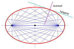
Orthogonal tangents

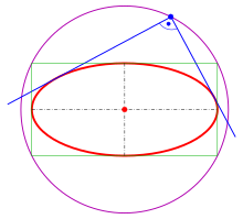
Ellipse with its orthoptic

For the ellipse x2a2+y2b2=1{displaystyle {tfrac {x^{2}}{a^{2}}}+{tfrac {y^{2}}{b^{2}}}=1}
the intersection points of orthogonal tangents lie on the circle x2+y2=a2+b2{displaystyle x^{2}+y^{2}=a^{2}+b^{2}}.

This circle is called orthoptic of the given ellipse.

Theorem of Apollonios on conjugate diameters

Ellipse: theorem of Apollonios on conjugate diameters

For an ellipse with semi-axes a,b{displaystyle a,;b} the following is true:

• Let c1{displaystyle c_{1}} and c2{displaystyle c_{2}} be halves of two conjugate diameters (see diagram) then

1. 
   c12+c22=a2+b2{displaystyle c_{1}^{2}+c_{2}^{2}=a^{2}+b^{2}},


2. the triangle formed by c1,c2{displaystyle c_{1},;c_{2}} has the constant area AΔ=12ab{displaystyle A_{Delta }={frac {1}{2}}ab}
   


3. the parallelogram of tangents adjacent to the given conjugate diameters has the Area12=4ab .{displaystyle {text{Area}}_{12}=4ab .}
   

Proof

Let the ellipse be in the canonical form with parametric equation

p→(t)=(acos⁡t,bsin⁡t)T{displaystyle {vec {p}}(t)=(acos t,bsin t)^{T}}.

The two points c→1=p→(t), c→2=p→(t+π/2){displaystyle {vec {c}}_{1}={vec {p}}(t), {vec {c}}_{2}={vec {p}}(t+pi /2)} are on conjugate diameters (see previous section). From trigonometric formulae one gets c→2=(−asin⁡t,bcos⁡t)T{displaystyle {vec {c}}_{2}=(-asin t,bcos t)^{T}} and

|c→1|2+|c→2|2=⋯=a2+b2 .{displaystyle |{vec {c}}_{1}|^{2}+|{vec {c}}_{2}|^{2}=cdots =a^{2}+b^{2} .}

The area of the triangle generated by c→1,c→2{displaystyle {vec {c}}_{1},{vec {c}}_{2}} is

AΔ=12det(c→1,c→2)=⋯=12ab{displaystyle A_{Delta }={tfrac {1}{2}}det({vec {c}}_{1},{vec {c}}_{2})=cdots ={tfrac {1}{2}}ab}

and from the diagram it can be seen that the area of the parallelogram is 8 times that of AΔ{displaystyle A_{Delta }}. Hence

Area12=4ab .{displaystyle {text{Area}}_{12}=4ab .}

Drawing ellipses

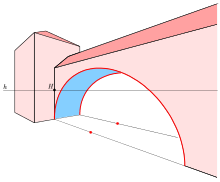
Central projection of circles (gate)

Ellipses appear in descriptive geometry as images (parallel or central projection) of circles. There exist various tools to draw an ellipse. Computers provide the fastest and most accurate method for drawing an ellipse. However, technical tools (ellipsographs) to draw an ellipse without a computer exist. The principle of ellipsographs were known to Greek mathematicians (Archimedes, Proklos).

If there is no ellipsograph available, the best and quickest way to draw an ellipse is to draw an Approximation by the four osculating circles at the vertices.

For any method described below

• the knowledge of the axes and the semi-axes is necessary (or equivalent: the foci and the semi-major axis).

If this presumption is not fulfilled one has to know at least two conjugate diameters. With help of Rytz's construction the axes and semi-axes can be retrieved.

de La Hire's point construction

The following construction of single points of an ellipse is due to de La Hire ^[4]. It is based on the standard parametric representation (acos⁡t,bsin⁡t){displaystyle (acos t,bsin t)} of an ellipse:

(1) Draw the two circles centered at the center of the ellipse with radii a,b{displaystyle a,b} and the axes of the ellipse.

(2) Draw a line through the center, which intersects the two circles at point A{displaystyle A} and B{displaystyle B}, respectively.

(3) The line through A{displaystyle A}, which is parallel to the minor axis, meets the line through B{displaystyle B}, which is parallel to the major axis, at an ellipse point (see diagram).

(4) Repeat steps (3) and (4) with different lines through the center.

• 
  

  

  
  

  
  

  de La Hire's method
  

  
  

  
  


• 
  

  

  
  

  
  

  Animation of the method
  

  
  

  
  

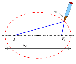
Ellipse: gardener's method

Pins-and-string method

The characterization of an ellipse as the locus of points so that sum of the distances to the foci is constant leads to a method of drawing one using two drawing pins, a length of string, and a pencil. In this method, pins are pushed into the paper at two points, which become the ellipse's foci. A string tied at each end to the two pins and the tip of a pencil pulls the loop taut to form a triangle. The tip of the pencil then traces an ellipse if it is moved while keeping the string taut. Using two pegs and a rope, gardeners use this procedure to outline an elliptical flower bed—thus it is called the gardener's ellipse.

A similar method for drawing confocal ellipses with a closed string is due to the Irish bishop Charles Graves.

Paper strip methods

The two following methods rely on the parametric representation (see section parametric representation, above):

(acos⁡t,bsin⁡t){displaystyle (acos t,;bsin t)}

This representation can be modeled technically by two simple methods. In both cases center, the axes and semi axes a,b{displaystyle a,;b} have to be known.

Method 1

The first method starts with

• a strip of paper of length a+b{displaystyle a+b}.

The point, where the semi axes meet is marked by P{displaystyle P}. If the strip slides with both ends on the axes of the desired ellipse, then point P traces the ellipse. For the proof one shows that point P{displaystyle P} has the parametric representation (acos⁡t,bsin⁡t){displaystyle (acos t,;bsin t)}, where parameter t{displaystyle t} is the angle of the slope of the paper strip.

A technical realization of the motion of the paper strip can be achieved by a Tusi couple (s. animation). The device is able to draw any ellipse with a fixed sum a+b{displaystyle a+b}, which is the radius of the large circle. This restriction may be a disadvantage in real life. More flexible is the second paper strip method.

A nice application: If one stands somewhere in the middle of a ladder, which stands on a slippery ground and leans on a slippery wall, the ladder slides down and the persons feet trace an ellipse.

• 
  

  

  
  

  
  

  Ellipse construction: paper strip method 1
  

  
  

  
  


• 
  

  

  
  

  
  

  Ellipses with Tusi couple. Two examples: red and cyan.
  

  
  

  
  

A variation of the paper strip method 1^[5] uses the observation that the midpoint N{displaystyle N} of the paper strip is moving on the circle with center M{displaystyle M} (of the ellipse) and radius a+b2{displaystyle {tfrac {a+b}{2}}}. Hence the paperstrip can be cut at point N{displaystyle N} into halves, connected again by a joint at N{displaystyle N} and the sliding end K{displaystyle K} fixed at the center M{displaystyle M} (see diagram). After this operation the movement of the unchanged half of the paperstrip is unchanged. The advantage of this variation is: Only one expensive sliding shoe is necessary.

One should be aware that the end, which is sliding on the minor axis, has to be changed.

• 
  

  

  
  

  
  

  Variation of the paper strip method 1
  

  
  

  
  


• 
  

  

  
  

  
  

  Animation of the variation of the paper strip method 1
  

  
  

  
  

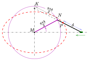
Ellipse construction: paper strip method 2

Method 2

The second method starts with

• a strip of paper of length a{displaystyle a}.

One marks the point, which divides the strip into two substrips of length b{displaystyle b} and a−b{displaystyle a-b}. The strip is positioned onto the axes as described in the diagram. Then the free end of the strip traces an ellipse, while the strip is moved. For the proof, one recognizes that the tracing point can be described parametrically by (acos⁡t,bsin⁡t){displaystyle (acos t,;bsin t)}, where parameter t{displaystyle t} is the angle of slope of the paper strip.

This method is the base for several ellipsographs (see section below).

Similar to the variation of the paper strip method 1 a variation of the paper strip method 2 can be established (see diagram) by cutting the part between the axes into halves.

• 
  

  

  
  

  
  

  Trammel of Archimedes (principle)
  

  
  

  
  


• 
  

  

  
  

  
  

  Ellipsograph due to Benjamin Bramer
  

  
  

  
  


• 
  

  

  
  

  
  

  Variation of the paper strip method 2
  

  
  

  
  

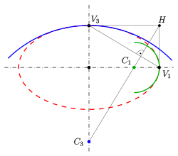
Approximation of an ellipse with osculating circles

Approximation by osculating circles

From section metric properties one gets:

• The radius of curvature at the vertices V1,V2{displaystyle V_{1},V_{2}} is: b2a ,{displaystyle {tfrac {b^{2}}{a}} ,}
  

the radius of curvature at the co-vertices V3,V4{displaystyle V_{3},V_{4}} is: a2b .{displaystyle {tfrac {a^{2}}{b}} .}

The diagram shows an easy way to find the centers C1=(a−b2a,0),C3=(0,b−a2b){displaystyle C_{1}=(a-{tfrac {b^{2}}{a}},0),;C_{3}=(0,b-{tfrac {a^{2}}{b}})} of curvature at vertex V1{displaystyle V_{1}} and co-vertex V3{displaystyle V_{3}}, respectively:

(1) mark the auxiliary point H=(a,b){displaystyle H=(a,b)} and draw the line segment V1V3 ,{displaystyle V_{1}V_{3} ,}

(2) draw the line through H{displaystyle H}, which is perpendicular to the line V1V3 ,{displaystyle V_{1}V_{3} ,}

(3) the intersection points of this line with the axes are the centers of the osculating circles.

(proof: simple calculation.)

The centers for the remaining vertices are found by symmetry.

With help of a French curve one draws a curve, which has smooth contact to the osculating circles.

Steiner generation of an ellipse

Ellipse: Steiner generation

Ellipse: Steiner generation

The following method to construct single points of an ellipse relies on the Steiner generation of a non degenerate conic section:

• Given two pencils B(U),B(V){displaystyle B(U),B(V)} of lines at two points U,V{displaystyle U,V} (all lines containing U{displaystyle U} and V{displaystyle V}, respectively) and a projective but not perspective mapping π{displaystyle pi } of B(U){displaystyle B(U)} onto B(V){displaystyle B(V)}, then the intersection points of corresponding lines form a non-degenerate projective conic section.

For the generation of points of the ellipse x2a2+y2b2=1{displaystyle {tfrac {x^{2}}{a^{2}}}+{tfrac {y^{2}}{b^{2}}}=1} one uses the pencils at the vertices V1,V2{displaystyle V_{1},V_{2}}. Let P=(0,b){displaystyle P=(0,b)} be an upper co-vertex of the ellipse and A=(−a,2b),B=(a,2b){displaystyle A=(-a,2b),B=(a,2b)}.
P{displaystyle P} is the center of the rectangle V1,V2,B,A{displaystyle V_{1},V_{2},B,A}. The side AB¯{displaystyle {overline {AB}}} of the rectangle is divided into n equal spaced line segments and this division is projected parallel with the diagonal AV2{displaystyle AV_{2}} as direction onto the line segment V1B¯{displaystyle {overline {V_{1}B}}} and assign the division as shown in the diagram. The parallel projection together with the reverse of the orientation is part of the projective mapping between the pencils at V1{displaystyle V_{1}} and V2{displaystyle V_{2}} needed. The intersection points of any two related lines V1Bi{displaystyle V_{1}B_{i}} and V2Ai{displaystyle V_{2}A_{i}} are points of the uniquely defined ellipse. With help of the points C1,…{displaystyle C_{1},dotsc } the points of the second quarter of the ellipse can be determined. Analogously one gets the points of the lower half of the ellipse.

The Steiner generation also exists for hyperbolas and parabolas. It is sometimes called a parallelogram method because one can use other points rather than the vertices, which starts with a parallelogram instead of a rectangle.

Ellipsographs

Most technical instruments for drawing ellipses are based on the second paperstrip method.

• Ellipsenzirkel (German)


• Drawing instruments

Inscribed angles for ellipses and the 3-point-form

Circles

Circle: inscribed angle theorem

A circle with equation (x−c)2+(y−d)2=r2, r>0 ,{displaystyle (x-c)^{2}+(y-d)^{2}=r^{2}, r>0 ,} is uniquely determined by three points (x1,y1),(x2,y2),(x3,y3){displaystyle (x_{1},y_{1}),;(x_{2},y_{2}),;(x_{3},y_{3})} not on a line. A simple way to determine the parameters c,d,r{displaystyle c,d,r} uses the inscribed angle theorem for circles:

For four points Pi=(xi,yi), i=1,2,3,4,{displaystyle P_{i}=(x_{i},y_{i}), i=1,2,3,4,} (see diagram) the following statement is true:

The four points are on a circle if and only if the angles at P3{displaystyle P_{3}} and P4{displaystyle P_{4}} are equal.

Usually one measures inscribed angles by degree or radian . In order to get an equation of a circle determined by three points, the following measurement is more convenient:

• In order to measure an angle between two lines with equations y=m1x+d1, y=m2x+d2 ,m1≠m2{displaystyle y=m_{1}x+d_{1}, y=m_{2}x+d_{2} ,m_{1}neq m_{2}} one uses the quotient

1+m1⋅m2m2−m1 .{displaystyle {frac {1+m_{1}cdot m_{2}}{m_{2}-m_{1}}} .}

This expression is the cotangent of the angle between the two lines.

Inscribed angle theorem for circles

For four points Pi=(xi,yi), i=1,2,3,4,{displaystyle P_{i}=(x_{i},y_{i}), i=1,2,3,4,}, no three of them on a line (see diagram), the following statement is true:

The four points are on a circle, if and only if the angles at P3{displaystyle P_{3}} and P4{displaystyle P_{4}} are equal. In the sense of the measurement above, that means, if

(x4−x1)(x4−x2)+(y4−y1)(y4−y2)(y4−y1)(x4−x2)−(y4−y2)(x4−x1)=(x3−x1)(x3−x2)+(y3−y1)(y3−y2)(y3−y1)(x3−x2)−(y3−y2)(x3−x1){displaystyle {frac {(x_{4}-x_{1})(x_{4}-x_{2})+(y_{4}-y_{1})(y_{4}-y_{2})}{(y_{4}-y_{1})(x_{4}-x_{2})-(y_{4}-y_{2})(x_{4}-x_{1})}}={frac {(x_{3}-x_{1})(x_{3}-x_{2})+(y_{3}-y_{1})(y_{3}-y_{2})}{(y_{3}-y_{1})(x_{3}-x_{2})-(y_{3}-y_{2})(x_{3}-x_{1})}}}

At first the measure is available for chords, which are not parallel to the y-axis, only. But the final formula works for any chord.

A consequence of the inscribed angle theorem for circles is the

3-point-form of a circle's equation

One gets the equation of the circle determined by 3 points Pi=(xi,yi){displaystyle P_{i}=(x_{i},y_{i})} not on a line by a conversion of the equation

(x−x1)(x−x2)+(y−y1)(y−y2)(y−y1)(x−x2)−(y−y2)(x−x1)=(x3−x1)(x3−x2)+(y3−y1)(y3−y2)(y3−y1)(x3−x2)−(y3−y2)(x3−x1) .{displaystyle {frac {({color {green}x}-x_{1})({color {green}x}-x_{2})+({color {red}y}-y_{1})({color {red}y}-y_{2})}{({color {red}y}-y_{1})({color {green}x}-x_{2})-({color {red}y}-y_{2})({color {green}x}-x_{1})}}={frac {(x_{3}-x_{1})(x_{3}-x_{2})+(y_{3}-y_{1})(y_{3}-y_{2})}{(y_{3}-y_{1})(x_{3}-x_{2})-(y_{3}-y_{2})(x_{3}-x_{1})}} .}

Using vectors, dot products and determinants this formula can be arranged more clearly:

(x→−x→1)⋅(x→−x→2)det(x→−x→1,x→−x→2)=(x→3−x→1)⋅(x→3−x→2)det(x→3−x→1,x→3−x→2).{displaystyle {frac {({color {red}{vec {x}}}-{vec {x}}_{1})cdot ({color {red}{vec {x}}}-{vec {x}}_{2})}{det({color {red}{vec {x}}}-{vec {x}}_{1},{color {red}{vec {x}}}-{vec {x}}_{2})}}={frac {({vec {x}}_{3}-{vec {x}}_{1})cdot ({vec {x}}_{3}-{vec {x}}_{2})}{det({vec {x}}_{3}-{vec {x}}_{1},{vec {x}}_{3}-{vec {x}}_{2})}};.}

For example, for P1=(2,0),P2=(0,1),P3=(0,0){displaystyle P_{1}=(2,0),;P_{2}=(0,1),;P_{3}=(0,0)} the 3-pointform is

(x−2)x+y(y−1)yx−(y−1)(x−2)=0{displaystyle {frac {(x-2)x+y(y-1)}{yx-(y-1)(x-2)}}=0}, which can be rearranged to (x−1)2+(y−1/2)2=5/4 .{displaystyle (x-1)^{2}+(y-1/2)^{2}=5/4 .}

Ellipses

This section considers ellipses with an equation

(x−c)2a2+(y−d)2b2=1↔(x−c)2+a2b2(y−d)2=a2,c,d,∈R, a>0 ,{displaystyle {frac {(x-c)^{2}}{a^{2}}}+{frac {(y-d)^{2}}{b^{2}}}=1quad leftrightarrow quad (x-c)^{2}+{frac {a^{2}}{b^{2}}}(y-d)^{2}=a^{2},quad c,d,in mathbb {R} , a>0 ,}

where the ratio a2b2{displaystyle {frac {a^{2}}{b^{2}}}} is fixed.
With the abbreviation q=a2b2 {displaystyle {color {blue}q}={frac {a^{2}}{b^{2}}} } one gets the more convenient form

• 
  (x−c)2+q(y−d)2=a2,c,d∈R,a>0{displaystyle (x-c)^{2}+{color {blue}q};(y-d)^{2}=a^{2},quad c,din mathbb {R} ,;a>0;} and q>0{displaystyle ;q>0;} fixed.

Such ellipses have their axes parallel to the coordinate axes and their eccentricity fixed. Their major axes are parallel to the x-axis if q>1{displaystyle q>1} and parallel to the y-axis if q<1{displaystyle q<1}.

Inscribed angle theorem for an ellipse

Like a circle, such an ellipse is determined by three points not on a line.

In this more general case one introduces the following measurement of an angle,:^[6][7]

• In order to measure an angle between two lines with equations y=m1x+d1, y=m2x+d2 ,m1≠m2{displaystyle y=m_{1}x+d_{1}, y=m_{2}x+d_{2} ,m_{1}neq m_{2}} one uses the quotient

1+qm1⋅m2m2−m1 .{displaystyle {frac {1+{color {blue}q};m_{1}cdot m_{2}}{m_{2}-m_{1}}} .}

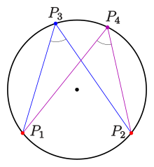
Inscribed angle theorem for ellipses

For four points Pi=(xi,yi), i=1,2,3,4,{displaystyle P_{i}=(x_{i},y_{i}), i=1,2,3,4,}, no three of them on a line (see diagram), the following statement is true:

The four points are on an ellipse with equation (x−c)2+q(y−d)2=a2{displaystyle (x-c)^{2}+q;(y-d)^{2}=a^{2}}, if and only if the angles at P3{displaystyle P_{3}} and P4{displaystyle P_{4}} are equal in the sense of the measurement above—that is, if

(x4−x1)(x4−x2)+q(y4−y1)(y4−y2)(y4−y1)(x4−x2)−(y4−y2)(x4−x1)=(x3−x1)(x3−x2)+q(y3−y1)(y3−y2)(y3−y1)(x3−x2)−(y3−y2)(x3−x1) .{displaystyle {frac {(x_{4}-x_{1})(x_{4}-x_{2})+{color {blue}q};(y_{4}-y_{1})(y_{4}-y_{2})}{(y_{4}-y_{1})(x_{4}-x_{2})-(y_{4}-y_{2})(x_{4}-x_{1})}}={frac {(x_{3}-x_{1})(x_{3}-x_{2})+{color {blue}q};(y_{3}-y_{1})(y_{3}-y_{2})}{(y_{3}-y_{1})(x_{3}-x_{2})-(y_{3}-y_{2})(x_{3}-x_{1})}} .}

At first the measure is available only for chords which are not parallel to the y-axis. But the final formula works for any chord. The proof follows from a straightforward calculation. For the direction of proof given that the points are on an ellipse, one can assume that the center of the ellipse is the origin.

A consequence of the inscribed angle theorem for ellipses is the

3-point-form of an ellipse's equation

One gets the equation of the ellipse determined by 3 points Pi=(xi,yi){displaystyle P_{i}=(x_{i},y_{i})} not on a line by a conversion of the equation

(x−x1)(x−x2)+q(y−y1)(y−y2)(y−y1)(x−x2)−(y−y2)(x−x1)=(x3−x1)(x3−x2)+q(y3−y1)(y3−y2)(y3−y1)(x3−x2)−(y3−y2)(x3−x1) .{displaystyle {frac {({color {green}x}-x_{1})({color {green}x}-x_{2})+{color {blue}q};({color {red}y}-y_{1})({color {red}y}-y_{2})}{({color {red}y}-y_{1})({color {green}x}-x_{2})-({color {red}y}-y_{2})({color {green}x}-x_{1})}}={frac {(x_{3}-x_{1})(x_{3}-x_{2})+{color {blue}q};(y_{3}-y_{1})(y_{3}-y_{2})}{(y_{3}-y_{1})(x_{3}-x_{2})-(y_{3}-y_{2})(x_{3}-x_{1})}} .}

Analogously to the circle case this formula can be written more clearly using vectors:

(x→−x→1)∗(x→−x→2)det(x→−x→1,x→−x→2)=(x→3−x→1)∗(x→3−x→2)det(x→3−x→1,x→3−x→2),{displaystyle {frac {({color {red}{vec {x}}}-{vec {x}}_{1})*({color {red}{vec {x}}}-{vec {x}}_{2})}{det({color {red}{vec {x}}}-{vec {x}}_{1},{color {red}{vec {x}}}-{vec {x}}_{2})}}={frac {({vec {x}}_{3}-{vec {x}}_{1})*({vec {x}}_{3}-{vec {x}}_{2})}{det({vec {x}}_{3}-{vec {x}}_{1},{vec {x}}_{3}-{vec {x}}_{2})}};,}

where ∗{displaystyle *} is the modified dot product u→∗v→=uxvx+quyvy.{displaystyle ;{vec {u}}*{vec {v}}=u_{x}v_{x}+{color {blue}q}u_{y}v_{y};.}

For example, for P1=(2,0),P2=(0,1),P3=(0,0){displaystyle P_{1}=(2,0),;P_{2}=(0,1),;P_{3}=(0,0)} and q=4{displaystyle q=4} one gets the 3-point-form

(x−2)x+4y(y−1)yx−(y−1)(x−2)=0{displaystyle {frac {(x-2)x+4y(y-1)}{yx-(y-1)(x-2)}}=0;} and after conversion (x−1)22+(y−1/2)21/2=1.{displaystyle ;{frac {(x-1)^{2}}{2}}+{frac {(y-1/2)^{2}}{1/2}}=1;.}

Pole-polar relation for an ellipse

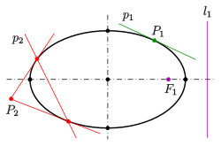
Ellipse: pole-polar relation

Any ellipse can be described in a suitable coordinate system by an equation x2a2+y2b2=1{displaystyle {tfrac {x^{2}}{a^{2}}}+{tfrac {y^{2}}{b^{2}}}=1}. The equation of the tangent at a point P0=(x0,y0){displaystyle P_{0}=(x_{0},y_{0})} of the ellipse is x0xa2+y0yb2=1.{displaystyle {tfrac {x_{0}x}{a^{2}}}+{tfrac {y_{0}y}{b^{2}}}=1.} If one allows point P0=(x0,y0){displaystyle P_{0}=(x_{0},y_{0})} to be an arbitrary point different from the origin, then

• point P0=(x0,y0)≠(0,0){displaystyle P_{0}=(x_{0},y_{0})neq (0,0)} is mapped onto the line x0xa2+y0yb2=1{displaystyle {frac {x_{0}x}{a^{2}}}+{frac {y_{0}y}{b^{2}}}=1}, not through the center of the ellipse.

This relation between points and lines is a bijection.

The inverse function maps

• line y=mx+d, d≠0{displaystyle y=mx+d, dneq 0} onto the point (−ma2d,b2d){displaystyle left(-{frac {ma^{2}}{d}},{frac {b^{2}}{d}}right)} and

line x=c, c≠0{displaystyle x=c, cneq 0} onto the point (a2c,0) .{displaystyle left({frac {a^{2}}{c}},0right) .}

Such a relation between points and lines generated by a conic is called pole-polar relation or just polarity. The pole is the point, the polar the line. See Pole and polar.

By calculation one can confirm the following properties of the pole-polar relation of the ellipse:

• For a point (pole) on the ellipse the polar is the tangent at this point (see diagram: P1, p1{displaystyle P_{1}, p_{1}}).


• For a pole P{displaystyle P} outside the ellipse the intersection points of its polar with the ellipse are the tangency points of the two tangents passing P{displaystyle P} (see diagram: P2, p2{displaystyle P_{2}, p_{2}}).


• For a point within the ellipse the polar has no point with the ellipse in common. (see diagram: F1, l1{displaystyle F_{1}, l_{1}}).

1. The intersection point of two polars is the pole of the line through their poles.


2. The foci (c,0),{displaystyle (c,0),} and (−c,0){displaystyle (-c,0)} respectively and the directrices x=a2c{displaystyle x={tfrac {a^{2}}{c}}} and x=−a2c{displaystyle x=-{tfrac {a^{2}}{c}}} respectively belong to pairs of pole and polar.

Pole-polar relations exist for hyperbolas and parabolas, too.

Metric properties

All metric properties given below refer to an ellipse with equation x2a2+y2b2=1{displaystyle {frac {x^{2}}{a^{2}}}+{frac {y^{2}}{b^{2}}}=1}.

Area

The area Aellipse{displaystyle A_{text{ellipse}}} enclosed by an ellipse is:

• Aellipse=πab{displaystyle A_{text{ellipse}}=pi ab}

where a{displaystyle a} and b{displaystyle b} are the lengths of the semi-major and semi-minor axes, respectively. The area formula πab{displaystyle pi ab} is intuitive: start with a circle of radius b{displaystyle b} (so its area is πb2{displaystyle pi b^{2}}) and stretch it by a factor a/b{displaystyle a/b} to make an ellipse. This scales the area by the same factor: πb2(a/b)=πab.{displaystyle pi b^{2}(a/b)=pi ab.} It is also easy to rigorously prove the area formula using integration as follows. Equation (1) can be rewritten as y(x)=b1−x2/a2.{displaystyle y(x)=b{sqrt {1-x^{2}/a^{2}}}.} For x∈[−a,a],{displaystyle xin [-a,a],} this curve is the top half of the ellipse. So twice the integral of y(x){displaystyle y(x)} over the interval [−a,a]{displaystyle [-a,a]} will be the area of the ellipse:

Aellipse=∫−aa2b1−x2/a2dx=ba∫−aa2a2−x2dx.{displaystyle {begin{aligned}A_{text{ellipse}}&=int _{-a}^{a}2b{sqrt {1-x^{2}/a^{2}}},dx\&={frac {b}{a}}int _{-a}^{a}2{sqrt {a^{2}-x^{2}}},dx.end{aligned}}}

The second integral is the area of a circle of radius a,{displaystyle a,} that is, πa2.{displaystyle pi a^{2}.} So

Aellipse=baπa2=πab.{displaystyle A_{text{ellipse}}={frac {b}{a}}pi a^{2}=pi ab.}

An ellipse defined implicitly by Ax2+Bxy+Cy2=1{displaystyle Ax^{2}+Bxy+Cy^{2}=1} has area 2π/4AC−B2.{displaystyle 2pi /{sqrt {4AC-B^{2}}}.}

The area can also be expressed in terms of eccentricity and the length of the semi-major axis as a2π1−e2{displaystyle a^{2}pi {sqrt {1-e^{2}}}} (obtained by solving for flattening, then computing the semi-minor axis).

Circumference

The circumference C{displaystyle C} of an ellipse is:

C=4a∫0π/21−e2sin2⁡θ dθ=4aE(e){displaystyle C=4aint _{0}^{pi /2}{sqrt {1-e^{2}sin ^{2}theta }} dtheta =4aE(e)}

where again a{displaystyle a} is the length of the semi-major axis, e{displaystyle e} is the eccentricity 1−b2/a2,{displaystyle {sqrt {1-b^{2}/a^{2}}},} and the function E{displaystyle E} is the complete elliptic integral of the second kind,

E(e)=∫0π/21−e2sin2⁡θ dθ.{displaystyle E(e)=int _{0}^{pi /2}{sqrt {1-e^{2}sin ^{2}theta }} dtheta .}

The circumference of the ellipse may be evaluated in terms of E(e){displaystyle E(e)} using Gauss's arithmetic-geometric mean;^[8] this is a quadratically converging iterative method.^[9]

The exact infinite series is:

C=2πa[1−(12)2e2−(1⋅32⋅4)2e43−(1⋅3⋅52⋅4⋅6)2e65−⋯]{displaystyle C=2pi aleft[{1-left({frac {1}{2}}right)^{2}e^{2}-left({frac {1cdot 3}{2cdot 4}}right)^{2}{frac {e^{4}}{3}}-left({frac {1cdot 3cdot 5}{2cdot 4cdot 6}}right)^{2}{frac {e^{6}}{5}}-cdots }right]}

=2πa[1−∑n=1∞((2n−1)!!(2n)!!)2e2n2n−1],{displaystyle =2pi aleft[1-sum _{n=1}^{infty }left({frac {(2n-1)!!}{(2n)!!}}right)^{2}{frac {e^{2n}}{2n-1}}right],}

where n!!{displaystyle n!!} is the double factorial. Unfortunately, this series converges rather slowly; however, by expanding in terms of h=(a−b)2/(a+b)2,{displaystyle h=(a-b)^{2}/(a+b)^{2},} Ivory^[10] and Bessel^[11] derived an expression that converges much more rapidly,

C=π(a+b)[1+∑n=1∞((2n−1)!!2nn!)2hn(2n−1)2].{displaystyle C=pi (a+b)left[1+sum _{n=1}^{infty }left({frac {(2n-1)!!}{2^{n}n!}}right)^{2}{frac {h^{n}}{(2n-1)^{2}}}right].}

Ramanujan gives two good approximations for the circumference in §16 of "Modular Equations and Approximations to π{displaystyle pi }";^[12] they are

C≈π[3(a+b)−(3a+b)(a+3b)]=π[3(a+b)−10ab+3(a2+b2)]{displaystyle Capprox pi left[3(a+b)-{sqrt {(3a+b)(a+3b)}}right]=pi left[3(a+b)-{sqrt {10ab+3(a^{2}+b^{2})}}right]}

and

C≈π(a+b)(1+3h10+4−3h).{displaystyle Capprox pi left(a+bright)left(1+{frac {3h}{10+{sqrt {4-3h}}}}right).}

The errors in these approximations, which were obtained empirically, are of order h3{displaystyle h^{3}} and h5,{displaystyle h^{5},} respectively.

More generally, the arc length of a portion of the circumference, as a function of the angle subtended, is given by an incomplete elliptic integral.

The inverse function, the angle subtended as a function of the arc length, is given by the elliptic functions.^{[citation needed]}

Some lower and upper bounds on the circumference of the canonical ellipse x2/a2+y2/b2=1{displaystyle x^{2}/a^{2}+y^{2}/b^{2}=1} with a≥b{displaystyle ageq b} are^[13]

2πb≤C≤2πa,{displaystyle 2pi bleq Cleq 2pi a,}

π(a+b)≤C≤4(a+b),{displaystyle pi (a+b)leq Cleq 4(a+b),}

4a2+b2≤C≤2πa2+b2.{displaystyle 4{sqrt {a^{2}+b^{2}}}leq Cleq {sqrt {2}}pi {sqrt {a^{2}+b^{2}}}.}

Here the upper bound 2πa{displaystyle 2pi a} is the circumference of a circumscribed concentric circle passing through the endpoints of the ellipse's major axis, and the lower bound 4a2+b2{displaystyle 4{sqrt {a^{2}+b^{2}}}} is the perimeter of an inscribed rhombus with vertices at the endpoints of the major and the minor axes.

Curvature

The curvature is given by κ=1a2b2(x2a4+y2b4)−32 ,{displaystyle kappa ={frac {1}{a^{2}b^{2}}}left({frac {x^{2}}{a^{4}}}+{frac {y^{2}}{b^{4}}}right)^{-{frac {3}{2}}} ,}
radius of curvature at point (x,y){displaystyle (x,y)}:

ρ=a2b2(x2a4+y2b4)3/2=1a4b4(a4y2+b4x2)3 .{displaystyle rho =a^{2}b^{2}left({frac {x^{2}}{a^{4}}}+{frac {y^{2}}{b^{4}}}right)^{3/2}={frac {1}{a^{4}b^{4}}}{sqrt {left(a^{4}y^{2}+b^{4}x^{2}right)^{3}}} .}

Radius of curvature at the two vertices (±a,0){displaystyle (pm a,0)} and the centers of curvature:

ρ0=b2a=p ,(±c2a|0) .{displaystyle rho _{0}={frac {b^{2}}{a}}=p ,qquad left(pm {frac {c^{2}}{a}},{bigg |},0right) .}

Radius of curvature at the two co-vertices (0,±b){displaystyle (0,pm b)} and the centers of curvature:

ρ1=a2b ,(0|±c2b) .{displaystyle rho _{1}={frac {a^{2}}{b}} ,qquad left(0,{bigg |},pm {frac {c^{2}}{b}}right) .}

Ellipse as quadric

General ellipse

In analytic geometry, the ellipse is defined as a quadric: the set of points (X,Y){displaystyle (X,Y)} of the Cartesian plane that, in non-degenerate cases, satisfy the implicit equation^[14][15]

 AX2+BXY+CY2+DX+EY+F=0{displaystyle ~AX^{2}+BXY+CY^{2}+DX+EY+F=0}

provided B2−4AC<0.{displaystyle B^{2}-4AC<0.}

To distinguish the degenerate cases from the non-degenerate case, let ∆ be the determinant

|AB/2D/2B/2CE/2D/2E/2F|;{displaystyle {begin{vmatrix}A&B/2&D/2\B/2&C&E/2\D/2&E/2&Fend{vmatrix}};}

that is,

Δ=(AC−B24)F+BED4−CD24−AE24.{displaystyle Delta =left(AC-{frac {B^{2}}{4}}right)F+{frac {BED}{4}}-{frac {CD^{2}}{4}}-{frac {AE^{2}}{4}}.}

Then the ellipse is a non-degenerate real ellipse if and only if C∆ < 0. If C∆ > 0, we have an imaginary ellipse, and if ∆ = 0, we have a point ellipse.^[16]:p.63

The general equation's coefficients can be obtained from known semi-major axis a{displaystyle a}, semi-minor axis b{displaystyle b}, center coordinates (xc,yc){displaystyle (x_{c},y_{c})} and rotation angle Θ{displaystyle Theta } using the following formulae:

A=a2(sin⁡Θ)2+b2(cos⁡Θ)2B=2(b2−a2)sin⁡Θcos⁡ΘC=a2(cos⁡Θ)2+b2(sin⁡Θ)2D=−2Axc−BycE=−Bxc−2CycF=Axc2+Bxcyc+Cyc2−a2b2{displaystyle {begin{aligned}A&=a^{2}(sin Theta )^{2}+b^{2}(cos Theta )^{2}\B&=2(b^{2}-a^{2})sin Theta cos Theta \C&=a^{2}(cos Theta )^{2}+b^{2}(sin Theta )^{2}\D&=-2Ax_{c}-By_{c}\E&=-Bx_{c}-2Cy_{c}\F&=Ax_{c}^{2}+Bx_{c}y_{c}+Cy_{c}^{2}-a^{2}b^{2}end{aligned}}}

These expressions can be derived from the canonical equation (see next section) by substituting the coordinates with expressions for rotation and translation of the coordinate system:

xcan2a2+ycan2b2=1{displaystyle {frac {x_{can}^{2}}{a^{2}}}+{frac {y_{can}^{2}}{b^{2}}}=1}

xcan=(x−xc)cos⁡Θ+(y−yc)sin⁡Θ{displaystyle x_{can}=(x-x_{c})cos Theta +(y-y_{c})sin Theta }

ycan=−(x−xc)sin⁡Θ+(y−yc)cos⁡Θ{displaystyle y_{can}=-(x-x_{c})sin Theta +(y-y_{c})cos Theta }

Canonical form

Let a>b{displaystyle a>b}. Through change of coordinates (a rotation of axes and a translation of axes) the general ellipse can be described by the canonical implicit equation

x2a2+y2b2=1{displaystyle {frac {x^{2}}{a^{2}}}+{frac {y^{2}}{b^{2}}}=1}

Here (x,y){displaystyle (x,y)} are the point coordinates in the canonical system, whose origin is the center (Xc,Yc){displaystyle (X_{c},Y_{c})} of the ellipse, whose x{displaystyle x}-axis is the unit vector (Xa,Ya){displaystyle (X_{a},Y_{a})} coinciding with the major axis, and whose y{displaystyle y}-axis is the perpendicular vector (−Ya,Xa){displaystyle (-Y_{a},X_{a})} coinciding with the minor axis. That is, x=Xa(X−Xc)+Ya(Y−Yc){displaystyle x=X_{a}(X-X_{c})+Y_{a}(Y-Y_{c})} and y=−Ya(X−Xc)+Xa(Y−Yc){displaystyle y=-Y_{a}(X-X_{c})+X_{a}(Y-Y_{c})}.

In this system, the center is the origin (0,0){displaystyle (0,0)} and the foci are (−ea,0){displaystyle (-ea,0)} and (+ea,0){displaystyle (+ea,0)} for eccentricity e.

Any ellipse can be obtained by rotation and translation of a canonical ellipse with the proper semi-diameters. The expression of an ellipse centered at (Xc,Yc){displaystyle (X_{c},Y_{c})} is

(x−Xc)2a2+(y−Yc)2b2=1{displaystyle {frac {(x-X_{c})^{2}}{a^{2}}}+{frac {(y-Y_{c})^{2}}{b^{2}}}=1}

Moreover, any canonical ellipse can be obtained by scaling the unit circle of R2{displaystyle mathbb {R} ^{2}}, defined by the equation

X2+Y2=1{displaystyle X^{2}+Y^{2}=1,}

by factors a and b along the two axes.

For an ellipse in canonical form, we have

Y=±b1−(X/a)2=±(a2−X2)(1−e2){displaystyle Y=pm b{sqrt {1-(X/a)^{2}}}=pm {sqrt {(a^{2}-X^{2})(1-e^{2})}}}

The distances from a point (X,Y){displaystyle (X,Y)} on the ellipse to the left and right foci are a+eX{displaystyle a+eX} and a−eX{displaystyle a-eX}, respectively.

The canonical form coefficients can be obtained from the general form coefficients using the following equations:

a,b=−2(AE2+CD2−BDE+(B2−4AC)F)(A+C±(A−C)2+B2)B2−4ACXc=2CD−BEB2−4ACYc=2AE−BDB2−4ACΘ={0for B=0,A<C90∘for B=0,A>Carctan⁡C−A−(A−C)2+B2Bfor B≠0{displaystyle {begin{aligned}a,b&={frac {-{sqrt {2{Big (}AE^{2}+CD^{2}-BDE+(B^{2}-4AC)F{Big )}left(A+Cpm {sqrt {(A-C)^{2}+B^{2}}}right)}}}{B^{2}-4AC}}\X_{c}&={frac {2CD-BE}{B^{2}-4AC}}\Y_{c}&={frac {2AE-BD}{B^{2}-4AC}}\Theta &={begin{cases}0&{text{for }}B=0,A<C\90^{circ }&{text{for }}B=0,A>C\arctan {frac {C-A-{sqrt {(A-C)^{2}+B^{2}}}}{B}}&{text{for }}Bneq 0end{cases}}end{aligned}}}

where Θ{displaystyle Theta } is the angle from the positive horizontal axis to the ellipse's major axis.

Polar forms

Polar form relative to center

Polar coordinates centered at the center

In polar coordinates, with the origin at the center of the ellipse and with the angular coordinate θ{displaystyle theta } measured from the major axis, the ellipse's equation is^{[16]:p. 75}

r(θ)=ab(bcos⁡θ)2+(asin⁡θ)2=b1−(ecos⁡θ)2{displaystyle r(theta )={frac {ab}{sqrt {(bcos theta )^{2}+(asin theta )^{2}}}}={frac {b}{sqrt {1-(ecos theta )^{2}}}}}

Polar form relative to focus

Polar coordinates centered at focus

If instead we use polar coordinates with the origin at one focus, with the angular coordinate θ=0{displaystyle theta =0} still measured from the major axis, the ellipse's equation is

r(θ)=a(1−e2)1±ecos⁡θ{displaystyle r(theta )={frac {a(1-e^{2})}{1pm ecos theta }}}

where the sign in the denominator is negative if the reference direction θ=0{displaystyle theta =0} points towards the center (as illustrated on the right), and positive if that direction points away from the center.

In the slightly more general case of an ellipse with one focus at the origin and the other focus at angular coordinate ϕ{displaystyle phi }, the polar form is

r=a(1−e2)1−ecos⁡(θ−ϕ).{displaystyle r={frac {a(1-e^{2})}{1-ecos(theta -phi )}}.}

The angle θ{displaystyle theta } in these formulas is called the true anomaly of the point. The numerator a(1−e2){displaystyle a(1-e^{2})} of these formulas is the semi-latus rectum of the ellipse, usually denoted l{displaystyle l}. It is the distance from a focus of the ellipse to the ellipse itself, measured along a line perpendicular to the major axis.

Ellipse as hypotrochoid

An ellipse (in red) as a special case of the hypotrochoid with R = 2r

The ellipse is a special case of the hypotrochoid when R = 2r, as shown in the adjacent image. The special case of a moving circle with radius r{displaystyle r} inside a circle with radius R=2r{displaystyle R=2r} is called a Tusi couple.

Ellipses in triangle geometry

Ellipses appear in triangle geometry as

1. 
   Steiner ellipse: ellipse through the vertices of the triangle with center at the centroid,


2. 
   inellipses: ellipses which touch the sides of a triangle. Special cases are the Steiner inellipse and the Mandart inellipse.

Ellipses as plane sections of quadrics

Ellipses appear as plane sections of the following quadrics:

• Ellipsoid


• Elliptic cone
  


• Elliptic cylinder
  


• Hyperboloid of one sheet


• Hyperboloid of two sheets

• 
  

  

  
  

  
  

  Ellipsoid
  

  
  

  
  


• 
  

  

  
  

  
  

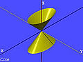
  Elliptic cone
  

  
  

  
  


• 
  

  

  
  

  
  

  Elliptic cylinder
  

  
  

  
  


• 
  

  

  
  

  
  

  Hyperboloid of one sheet
  

  
  

  
  


• 
  

  

  
  

  
  

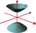
  Hyperboloid of two sheets
  

  
  

  
  

Applications

Physics

Elliptical reflectors and acoustics

If the water's surface is disturbed at one focus of an elliptical water tank, the circular waves of that disturbance, after reflecting off the walls, converge simultaneously to a single point: the second focus. This is a consequence of the total travel length being the same along any wall-bouncing path between the two foci.

Similarly, if a light source is placed at one focus of an elliptic mirror, all light rays on the plane of the ellipse are reflected to the second focus. Since no other smooth curve has such a property, it can be used as an alternative definition of an ellipse. (In the special case of a circle with a source at its center all light would be reflected back to the center.) If the ellipse is rotated along its major axis to produce an ellipsoidal mirror (specifically, a prolate spheroid), this property holds for all rays out of the source. Alternatively, a cylindrical mirror with elliptical cross-section can be used to focus light from a linear fluorescent lamp along a line of the paper; such mirrors are used in some document scanners.

Sound waves are reflected in a similar way, so in a large elliptical room a person standing at one focus can hear a person standing at the other focus remarkably well. The effect is even more evident under a vaulted roof shaped as a section of a prolate spheroid. Such a room is called a whisper chamber. The same effect can be demonstrated with two reflectors shaped like the end caps of such a spheroid, placed facing each other at the proper distance. Examples are the National Statuary Hall at the United States Capitol (where John Quincy Adams is said to have used this property for eavesdropping on political matters); the Mormon Tabernacle at Temple Square in Salt Lake City, Utah; at an exhibit on sound at the Museum of Science and Industry in Chicago; in front of the University of Illinois at Urbana–Champaign Foellinger Auditorium; and also at a side chamber of the Palace of Charles V, in the Alhambra.

Planetary orbits

In the 17th century, Johannes Kepler discovered that the orbits along which the planets travel around the Sun are ellipses with the Sun [approximately] at one focus, in his first law of planetary motion. Later, Isaac Newton explained this as a corollary of his law of universal gravitation.

More generally, in the gravitational two-body problem, if the two bodies are bound to each other (that is, the total energy is negative), their orbits are similar ellipses with the common barycenter being one of the foci of each ellipse. The other focus of either ellipse has no known physical significance. The orbit of either body in the reference frame of the other is also an ellipse, with the other body at the same focus.

Keplerian elliptical orbits are the result of any radially directed attraction force whose strength is inversely proportional to the square of the distance. Thus, in principle, the motion of two oppositely charged particles in empty space would also be an ellipse. (However, this conclusion ignores losses due to electromagnetic radiation and quantum effects, which become significant when the particles are moving at high speed.)

For elliptical orbits, useful relations involving the eccentricity e{displaystyle e} are:

e=ra−rpra+rp=ra−rp2ara=(1+e)arp=(1−e)a{displaystyle {begin{aligned}e&={frac {r_{a}-r_{p}}{r_{a}+r_{p}}}={frac {r_{a}-r_{p}}{2a}}\r_{a}&=(1+e)a\r_{p}&=(1-e)aend{aligned}}}

where

• 
  ra{displaystyle r_{a}} is the radius at apoapsis (the farthest distance)


• 
  rp{displaystyle r_{p}} is the radius at periapsis (the closest distance)


• 
  a{displaystyle a} is the length of the semi-major axis
  

Also, in terms of ra{displaystyle r_{a}} and rp{displaystyle r_{p}}, the semi-major axis a{displaystyle a} is their arithmetic mean, the semi-minor axis b{displaystyle b} is their geometric mean, and the semi-latus rectum l{displaystyle l} is their harmonic mean. In other words,

a=ra+rp2b=ra⋅rpl=21ra+1rp=2rarpra+rp{displaystyle {begin{aligned}a&={frac {r_{a}+r_{p}}{2}}\b&={sqrt {r_{a}cdot r_{p}}}\l&={frac {2}{{frac {1}{r_{a}}}+{frac {1}{r_{p}}}}}={frac {2r_{a}r_{p}}{r_{a}+r_{p}}}end{aligned}}}.

Harmonic oscillators

The general solution for a harmonic oscillator in two or more dimensions is also an ellipse. Such is the case, for instance, of a long pendulum that is free to move in two dimensions; of a mass attached to a fixed point by a perfectly elastic spring; or of any object that moves under influence of an attractive force that is directly proportional to its distance from a fixed attractor. Unlike Keplerian orbits, however, these "harmonic orbits" have the center of attraction at the geometric center of the ellipse, and have fairly simple equations of motion.

Phase visualization

In electronics, the relative phase of two sinusoidal signals can be compared by feeding them to the vertical and horizontal inputs of an oscilloscope. If the display is an ellipse, rather than a straight line, the two signals are out of phase.

Elliptical gears

Two non-circular gears with the same elliptical outline, each pivoting around one focus and positioned at the proper angle, turn smoothly while maintaining contact at all times. Alternatively, they can be connected by a link chain or timing belt, or in the case of a bicycle the main chainring may be elliptical, or an ovoid similar to an ellipse in form. Such elliptical gears may be used in mechanical equipment to produce variable angular speed or torque from a constant rotation of the driving axle, or in the case of a bicycle to allow a varying crank rotation speed with inversely varying mechanical advantage.

Elliptical bicycle gears make it easier for the chain to slide off the cog when changing gears.^[17]

An example gear application would be a device that winds thread onto a conical bobbin on a spinning machine. The bobbin would need to wind faster when the thread is near the apex than when it is near the base.^[18]

Optics

• In a material that is optically anisotropic (birefringent), the refractive index depends on the direction of the light. The dependency can be described by an index ellipsoid. (If the material is optically isotropic, this ellipsoid is a sphere.)


• In lamp-pumped solid-state lasers, elliptical cylinder-shaped reflectors have been used to direct light from the pump lamp (coaxial with one ellipse focal axis) to the active medium rod (coaxial with the second focal axis).^[19]
  


• In laser-plasma produced EUV light sources used in microchip lithography, EUV light is generated by plasma positioned in the primary focus of an ellipsoid mirror and is collected in the secondary focus at the input of the lithography machine.^[20]
  

Statistics and finance

In statistics, a bivariate random vector (X, Y) is jointly elliptically distributed if its iso-density contours—loci of equal values of the density function—are ellipses. The concept extends to an arbitrary number of elements of the random vector, in which case in general the iso-density contours are ellipsoids. A special case is the multivariate normal distribution. The elliptical distributions are important in finance because if rates of return on assets are jointly elliptically distributed then all portfolios can be characterized completely by their mean and variance—that is, any two portfolios with identical mean and variance of portfolio return have identical distributions of portfolio return.^[21][22]

Computer graphics

Drawing an ellipse as a graphics primitive is common in standard display libraries, such as the MacIntosh QuickDraw API, and Direct2D on Windows. Jack Bresenham at IBM is most famous for the invention of 2D drawing primitives, including line and circle drawing, using only fast integer operations such as addition and branch on carry bit. M. L. V. Pitteway extended Bresenham's algorithm for lines to conics in 1967.^[23] Another efficient generalization to draw ellipses was invented in 1984 by Jerry Van Aken.^[24]

In 1970 Danny Cohen presented at the "Computer Graphics 1970" conference in England a linear algorithm for drawing ellipses and circles. In 1971, L. B. Smith published similar algorithms for all conic sections and proved them to have good properties.^[25] These algorithms need only a few multiplications and additions to calculate each vector.

It is beneficial to use a parametric formulation in computer graphics because the density of points is greatest where there is the most curvature. Thus, the change in slope between each successive point is small, reducing the apparent "jaggedness" of the approximation.

Drawing with Bézier paths

Composite Bézier curves may also be used to draw an ellipse to sufficient accuracy, since any ellipse may be construed as an affine transformation of a circle. The spline methods used to draw a circle may be used to draw an ellipse, since the constituent Bézier curves behave appropriately under such transformations.

Optimization theory

It is sometimes useful to find the minimum bounding ellipse on a set of points. The ellipsoid method is quite useful for attacking this problem.

See also

Notes

References

• 
  Besant, W.H. (1907). "Chapter III. The Ellipse". Conic Sections. London: George Bell and Sons. p. 50.
  


• 
  Coxeter, H.S.M. (1969). Introduction to Geometry (2nd ed.). New York: Wiley. pp. 115–9.
  


• 
  Meserve, Bruce E. (1983) [1959], Fundamental Concepts of Geometry, Dover, ISBN 978-0-486-63415-9
  


• 
  Miller, Charles D.; Lial, Margaret L.; Schneider, David I. (1990). Fundamentals of College Algebra (3rd ed.). Scott Foresman/Little. p. 381. ISBN 978-0-673-38638-0.
  

External links

• 
  Quotations related to Ellipse at Wikiquote


• 
  Media related to Ellipses at Wikimedia Commons


• 
  Ellipse (mathematics) at Encyclopædia Britannica
  


• 
  ellipse at PlanetMath.org.


• Weisstein, Eric W. "Ellipse". MathWorld.


• Weisstein, Eric W. "Ellipse as special case of hypotrochoid". MathWorld.


• 
  Apollonius' Derivation of the Ellipse at Convergence


• 
  The Shape and History of The Ellipse in Washington, D.C. by Clark Kimberling
  


• Ellipse circumference calculator


• Collection of animated ellipse demonstrations


• 
  Ivanov, A.B. (2001) [1994], "Ellipse", in Hazewinkel, Michiel, Encyclopedia of Mathematics, Springer Science+Business Media B.V. / Kluwer Academic Publishers, ISBN 978-1-55608-010-4
  


• Trammel according Frans van Schooten