Agfdhyk

Part of a series of articles about
Electromagnetism
Electricity Magnetism
Electrostatics Conductor Coulomb's law Electric charge Electric dipole moment Electric field Electric flux / potential energy Electrostatic discharge Gauss's law Induction Insulator Polarization density Static electricity Triboelectricity
Magnetostatics Ampère's law Biot–Savart law Gauss's law for magnetism Magnetic field Magnetic flux Magnetic dipole moment Magnetization Magnetomotive force
Electrodynamics Lorentz force law Electromagnetic induction Faraday's law Lenz's law Displacement current Magnetic potential Maxwell's equations Electromagnetic field Electromagnetic pulse Electromagnetic radiation Maxwell tensor Poynting vector Liénard–Wiechert potential Jefimenko's equations Eddy current London equations Mathematical descriptions of the electromagnetic field
Electrical network Alternating current Capacitance Direct current Electric current Electric potential Electromotive force Impedance Inductance Ohm's law Parallel circuit Resistance Resonant cavities Series circuit Voltage Waveguides
Covariant formulation Electromagnetic tensor (stress–energy tensor) Four-current Electromagnetic four-potential
Scientists Ampère Coulomb Faraday Gauss Heaviside Henry Hertz Lorentz Maxwell Ørsted Tesla Volta Weber
v t e

Coulomb's law, or Coulomb's inverse-square law, is an experimental law^[1] of physics that quantifies the amount of force between two stationary, electrically charged particles. The electric force between charged bodies at rest is conventionally called electrostatic force^[2] or Coulomb force.^[3] The quantity of electrostatic force between stationary charges is always described by Coulomb’s law.^[4] The law was first published in 1785 by French physicist Charles-Augustin de Coulomb, and was essential to the development of the theory of electromagnetism, maybe even its starting point,^[5] because it was now possible to discuss quantity of electric charge in a meaningful way.^[6]

In its scalar form, the law is:

F=keq1q2r2,{displaystyle F=k_{e}{frac {q_{1}q_{2}}{r^{2}}},}

where k_e is Coulomb's constant (k_e ≈ 7009900000000000000♠9×10⁹ N⋅m²⋅C⁻²),^[7]q₁ and q₂ are the signed magnitudes of the charges, and the scalar r is the distance between the charges. The force of the interaction between the charges is attractive if the charges have opposite signs (i.e., F is negative) and repulsive if like-signed (i.e., F is positive).

Being an inverse-square law, the law is analogous to Isaac Newton's inverse-square law of universal gravitation, but gravitational forces are always attractive, while electrostatic forces can be attractive or repulsive.^[8] Coulomb's law can be used to derive Gauss's law, and vice versa. The two laws are equivalent, expressing the same physical law in different ways.^[9] The law has been tested extensively, and observations have upheld the law on a scale from 10⁻¹⁶ m to 10⁸ m.^[10]

History

Charles-Augustin de Coulomb

Ancient cultures around the Mediterranean knew that certain objects, such as rods of amber, could be rubbed with cat's fur to attract light objects like feathers. Thales of Miletus made a series of observations on static electricity around 600 BC, from which he believed that friction rendered amber magnetic, in contrast to minerals such as magnetite, which needed no rubbing.^[11][12] Thales was incorrect in believing the attraction was due to a magnetic effect, but later science would prove a link between magnetism and electricity. Electricity would remain little more than an intellectual curiosity for millennia until 1600, when the English scientist William Gilbert made a careful study of electricity and magnetism, distinguishing the lodestone effect from static electricity produced by rubbing amber.^[11] He coined the New Latin word electricus ("of amber" or "like amber", from ἤλεκτρον [elektron], the Greek word for "amber") to refer to the property of attracting small objects after being rubbed.^[13] This association gave rise to the English words "electric" and "electricity", which made their first appearance in print in Thomas Browne's Pseudodoxia Epidemica of 1646.^[14]

Early investigators of the 18th century who suspected that the electrical force diminished with distance as the force of gravity did (i.e., as the inverse square of the distance) included Daniel Bernoulli^[15] and Alessandro Volta, both of whom measured the force between plates of a capacitor, and Franz Aepinus who supposed the inverse-square law in 1758.^[16]

Based on experiments with electrically charged spheres, Joseph Priestley of England was among the first to propose that electrical force followed an inverse-square law, similar to Newton's law of universal gravitation. However, he did not generalize or elaborate on this.^[17] In 1767, he conjectured that the force between charges varied as the inverse square of the distance.^[18][19]

Coulomb's torsion balance

In 1769, Scottish physicist John Robison announced that, according to his measurements, the force of repulsion between two spheres with charges of the same sign varied as x^−2.06.^[20]

In the early 1770s, the dependence of the force between charged bodies upon both distance and charge had already been discovered, but not published, by Henry Cavendish of England.^[21]

Finally, in 1785, the French physicist Charles-Augustin de Coulomb published his first three reports of electricity and magnetism where he stated his law. This publication was essential to the development of the theory of electromagnetism.^[22] He used a torsion balance to study the repulsion and attraction forces of charged particles, and determined that the magnitude of the electric force between two point charges is directly proportional to the product of the charges and inversely proportional to the square of the distance between them.

The torsion balance consists of a bar suspended from its middle by a thin fiber. The fiber acts as a very weak torsion spring. In Coulomb's experiment, the torsion balance was an insulating rod with a metal-coated ball attached to one end, suspended by a silk thread. The ball was charged with a known charge of static electricity, and a second charged ball of the same polarity was brought near it. The two charged balls repelled one another, twisting the fiber through a certain angle, which could be read from a scale on the instrument. By knowing how much force it took to twist the fiber through a given angle, Coulomb was able to calculate the force between the balls and derive his inverse-square proportionality law.

The law

Coulomb's law states that:

The magnitude of the electrostatic force of attraction or repulsion between two point charges is directly proportional to the product of the magnitudes of charges and inversely proportional to the square of the distance between them.^[22]

The force is along the straight line joining them. If the two charges have the same sign, the electrostatic force between them is repulsive; if they have different signs, the force between them is attractive.

Coulomb's law can also be stated as a simple mathematical expression. The scalar and vector forms of the mathematical equation are

|F|=ke|q1q2|r2{displaystyle |mathbf {F} |=k_{e}{|q_{1}q_{2}| over r^{2}}qquad } and F1=keq1q2|r21|2r^21,{displaystyle qquad mathbf {F} _{1}=k_{e}{frac {q_{1}q_{2}}{{|mathbf {r} _{21}|}^{2}}}mathbf {widehat {r}} _{21},qquad } respectively,

where k_e is Coulomb's constant (k_e = 7009898755178736817♠8.9875517873681764×10⁹ N⋅m²⋅C⁻²), q₁ and q₂ are the signed magnitudes of the charges, the scalar r is the distance between the charges, the vector r₂₁ = r₁ − r₂ is the vectorial distance between the charges, and r̂₂₁ = r₂₁/|r₂₁| (a unit vector pointing from q₂ to q₁). The vector form of the equation calculates the force F₁ applied on q₁ by q₂. If r₁₂ is used instead, then the effect on q₂ can be found. It can be also calculated using Newton's third law: F₂ = −F₁.

Units

When the electromagnetic theory is expressed in the International System of Units, force is measured in newtons, charge in coulombs, and distance in meters. Coulomb's constant is given by k_e = 1/4πε₀. The constant ε₀ is the vacuum electric permittivity (also known as "electric constant") ^[23] in C²⋅m⁻²⋅N⁻¹. It should not be confused with ε_r, which is the dimensionless relative permittivity of the material in which the charges are immersed, or with their product ε_a = ε₀ε_r, which is called "absolute permittivity of the material" and is still used in electrical engineering.

The SI derived units for the electric field are volts per meter, newtons per coulomb, or tesla meters per second.

Coulomb's law and Coulomb's constant can also be interpreted in various terms:

• 
  Atomic units. In atomic units the force is expressed in hartrees per Bohr radius, the charge in terms of the elementary charge, and the distances in terms of the Bohr radius.


• 
  Electrostatic units or Gaussian units. In electrostatic units and Gaussian units, the unit charge (esu or statcoulomb) is defined in such a way that the Coulomb constant k disappears because it has the value of one and becomes dimensionless.


• 
  Lorentz–Heaviside units (also called rationalized). In Lorentz–Heaviside units the Coulomb constant is k_e = 1/4π and becomes dimensionless.

Gaussian units and Lorentz–Heaviside units are both CGS unit systems. Gaussian units are more amenable for microscopic problems such as the electrodynamics of individual electrically charged particles.^[24] SI units are more convenient for practical, large-scale phenomena, such as engineeering applications.^[24]

Electric field

If two charges have the same sign, the electrostatic force between them is repulsive; if they have different sign, the force between them is attractive.

An electric field is a vector field that associates to each point in space the Coulomb force experienced by a test charge. In the simplest case, the field is considered to be generated solely by a single source point charge. The strength and direction of the Coulomb force F on a test charge q_t depends on the electric field E that it finds itself in, such that F = q_tE. If the field is generated by a positive source point charge q, the direction of the electric field points along lines directed radially outwards from it, i.e. in the direction that a positive point test charge q_t would move if placed in the field. For a negative point source charge, the direction is radially inwards.

The magnitude of the electric field E can be derived from Coulomb's law. By choosing one of the point charges to be the source, and the other to be the test charge, it follows from Coulomb's law that the magnitude of the electric field E created by a single source point charge q at a certain distance from it r in vacuum is given by:

|E|=14πε0|q|r2{displaystyle |{boldsymbol {E}}|={1 over 4pi varepsilon _{0}}{|q| over r^{2}}}

Coulomb's constant

Coulomb's constant is a proportionality factor that appears in Coulomb's law as well as in other electric-related formulas. Denoted k_e, it is also called the electric force constant or electrostatic constant,^[8] hence the subscript e.

The exact value of Coulomb's constant is:

ke=14πε0=c02μ04π=c02×10−7 H⋅m−1=8.9875517873681764×109 N⋅m2⋅C−2{displaystyle {begin{aligned}k_{e}&={frac {1}{4pi varepsilon _{0}}}={frac {c_{0}^{2}mu _{0}}{4pi }}=c_{0}^{2}times 10^{-7} mathrm {Hcdot m} ^{-1}\&=8.987,551,787,368,176,4times 10^{9} mathrm {Ncdot m^{2}cdot C} ^{-2}end{aligned}}}

Limitations

There are three conditions to be fulfilled for the validity of Coulomb's law:

1. The charges must have a spherically symmetric distribution (e.g. be point charges, or a charged metal sphere).


2. The charges must not overlap (e.g. they must be distinct point charges).


3. The charges must be stationary with respect to each other.

The last of these is known as the electrostatic approximation. When movement takes place, Einstein's theory of relativity must be taken into consideration, and a result, an extra factor is introduced, which alters the force produced on the two objects. This extra part of the force is called the magnetic force, and is described by magnetic fields. For slow movement, the magnetic force is minimal and Coulomb's law can still be considered approximately correct, but when the charges are moving more quickly in relation to each other, the full electrodynamic rules (incorporating the magnetic force) must be considered.

Quantum field theory origin

The most basic Feynman diagram for QED interaction between two fermions

In simple terms, the Coulomb potential derives from the QED Lagrangian as follows. The Lagrangian of quantum electrodynamics is normally written in natural units, but in SI units, it is:

LQED=ψ¯(iℏcγμDμ−mc2)ψ−14ℏcFμνFμν{displaystyle {mathcal {L}}_{mathrm {QED} }={bar {psi }}(ihbar cgamma ^{mu }D_{mu }-mc^{2})psi -{frac {1}{4hbar c}}F_{mu nu }F^{mu nu }}

where the covariant derivative (in SI units) is:

Dμ=∂μ+igℏcAμ{displaystyle {D}_{mu }=partial _{mu }+{frac {ig}{hbar c}}A_{mu }}

where g{displaystyle g} is the gauge coupling parameter. By putting the covariant derivative into the lagrangian explicitly, the interaction term (the term involving both A{displaystyle A} and ψ{displaystyle psi }) is seen to be:

Lint=igψ¯γμAμψ{displaystyle {mathcal {L}}_{mathrm {int} }=ig{bar {psi }}gamma ^{mu }A_{mu }psi }

The most basic Feynman diagram for a QED interaction between two fermions is the exchange of a single photon, with no loops. Following the Feynman rules, this therefore contributes two QED vertex factors (igQγμ{displaystyle igQgamma _{mu }}) to the potential, where Q is the QED-charge operator (Q gives the charge in terms of the electron charge, and hence is exactly −1 for electrons, etc.). For the photon in the diagram, the Feynman rules demand the contribution of one bosonic massless propagator (ℏck2){displaystyle left({frac {hbar c}{k^{2}}}right)}. Ignoring the momentum on the external legs (the fermions), the potential is therefore:

V(r)=1(2π)3∫eik⋅rℏ(iQ1g2γμ)(iQ2g2γν)(ℏck2)d3k{displaystyle V(mathbf {r} )={frac {1}{(2pi )^{3}}}int e^{frac {imathbf {kcdot r} }{hbar }}(iQ_{1}g^{2}gamma _{mu })(iQ_{2}g^{2}gamma _{nu })left({frac {hbar c}{k^{2}}}right);d^{3}k}

which can be more usefully written as

V(r)=−g2ℏcQ1Q24π1(2π)3∫eik⋅rℏ4πημνk2d3k{displaystyle V(mathbf {r} )={frac {-g^{2}hbar cQ_{1}Q_{2}}{4pi }}{frac {1}{(2pi )^{3}}}int e^{frac {imathbf {kcdot r} }{hbar }}{frac {4pi eta _{mu nu }}{k^{2}}};d^{3}k}

where Qi{displaystyle Q_{i}} is the QED-charge on the ith particle. Recognising the integral as just being a Fourier transform enables the equation to be simplified:

V(r)=−g2ℏcQ1Q24π1r.{displaystyle V(mathbf {r} )={frac {-g^{2}hbar cQ_{1}Q_{2}}{4pi }}{frac {1}{r}}.}

For various reasons, it is more convenient to define the fine-structure constant α=g24π{displaystyle alpha ={frac {g^{2}}{4pi }}}, and then define e=4παε0ℏc{displaystyle e={sqrt {4pi alpha varepsilon _{0}hbar c}}}. Rearranging these definitions gives:

g2ℏc=e2ε0{displaystyle g^{2}hbar c={frac {e^{2}}{varepsilon _{0}}}}

It is worth noting that g=e{displaystyle g=e} in natural units (since, in those units, ℏ=1{displaystyle hbar =1}, c=1{displaystyle c=1}, and ε0=1{displaystyle varepsilon _{0}=1}). Continuing in SI units, the potential is therefore

V(r)=−e24πε0Q1Q2r{displaystyle V(mathbf {r} )={frac {-e^{2}}{4pi varepsilon _{0}}}{frac {Q_{1}Q_{2}}{r}}}

Defining qi=eQi{displaystyle q_{i}=eQ_{i}}, as the macroscopic 'electric charge', makes e the macroscopic 'electric charge' for an electron, and enables the formula to be put into the familiar form of the Coulomb potential:

V(r)=−14πε0q1q2r{displaystyle V(mathbf {r} )={frac {-1}{4pi varepsilon _{0}}}{frac {q_{1}q_{2}}{r}}}

The force (dV(r)dr{displaystyle {frac {dV(mathbf {r} )}{dr}}}) is therefore :

F(r)=14πε0q1q2r2{displaystyle F(mathbf {r} )={frac {1}{4pi varepsilon _{0}}}{frac {q_{1}q_{2}}{r^{2}}}}

The derivation makes clear that the force law is only an approximation — it ignores the momentum of the input and output fermion lines, and ignores all quantum corrections (ie. the myriad possible diagrams with internal loops).

The Coulomb potential, and its derivation, can be seen as a special case of the Yukawa potential (specifically, the case where the exchanged boson – the photon – has no rest mass).

Scalar form

The absolute value of the force F between two point charges q and Q relates to the distance between the point charges and to the simple product of their charges. The diagram shows that like charges repel each other, and opposite charges mutually attract.

When it is of interest to know the magnitude of the electrostatic force (and not its direction), it may be easiest to consider a scalar version of the law. The scalar form of Coulomb's Law relates the magnitude and sign of the electrostatic force F acting simultaneously on two point charges q₁ and q₂ as follows:

|F|=ke|q1q2|r2{displaystyle |{boldsymbol {F}}|=k_{e}{|q_{1}q_{2}| over r^{2}}}

where r is the separation distance and k_e is Coulomb's constant. If the product q₁q₂ is positive, the force between the two charges is repulsive; if the product is negative, the force between them is attractive.^[25]

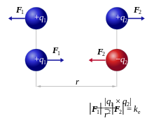
Vector form

In the image, the vector F₁ is the force experienced by q₁, and the vector F₂ is the force experienced by q₂. When q₁q₂ > 0 the forces are repulsive (as in the image) and when q₁q₂ < 0 the forces are attractive (opposite to the image). The magnitude of the forces will always be equal.

Coulomb's law states that the electrostatic force F₁ experienced by a charge, q₁ at position r₁, in the vicinity of another charge, q₂ at position r₂, in a vacuum is equal to:

F1=q1q24πε0(r1−r2)|r1−r2|3=q1q24πε0r^21|r21|2,{displaystyle {boldsymbol {F_{1}}}={q_{1}q_{2} over 4pi varepsilon _{0}}{({boldsymbol {r_{1}-r_{2}}}) over |{boldsymbol {r_{1}-r_{2}}}|^{3}}={q_{1}q_{2} over 4pi varepsilon _{0}}{{boldsymbol {{widehat {r}}_{21}}} over |{boldsymbol {r_{21}}}|^{2}},}

where r₂₁ = r₁ − r₂, the unit vector r̂₂₁ = r₂₁/|r₂₁|, and ε₀ is the electric constant.

The vector form of Coulomb's law is simply the scalar definition of the law with the direction given by the unit vector, r̂₂₁, parallel with the line from charge q₂ to charge q₁.^[26] If both charges have the same sign (like charges) then the product q₁q₂ is positive and the direction of the force on q₁ is given by r̂₂₁; the charges repel each other. If the charges have opposite signs then the product q₁q₂ is negative and the direction of the force on q₁ is given by −r̂₂₁ = r̂₁₂; the charges attract each other.

The electrostatic force F₂ experienced by q₂, according to Newton's third law, is F₂ = −F₁.

System of discrete charges

The law of superposition allows Coulomb's law to be extended to include any number of point charges. The force acting on a point charge due to a system of point charges is simply the vector addition of the individual forces acting alone on that point charge due to each one of the charges. The resulting force vector is parallel to the electric field vector at that point, with that point charge removed.

The force F on a small charge q at position r, due to a system of N discrete charges in vacuum is:

F(r)=q4πε0∑i=1Nqir−ri|r−ri|3=q4πε0∑i=1NqiRi^|Ri|2,{displaystyle {boldsymbol {F(r)}}={q over 4pi varepsilon _{0}}sum _{i=1}^{N}q_{i}{{boldsymbol {r-r_{i}}} over |{boldsymbol {r-r_{i}}}|^{3}}={q over 4pi varepsilon _{0}}sum _{i=1}^{N}q_{i}{{boldsymbol {widehat {R_{i}}}} over |{boldsymbol {R_{i}}}|^{2}},}

where q_i and r_i are the magnitude and position respectively of the ith charge, R̂_i is a unit vector in the direction of R_i = r − r_i (a vector pointing from charges q_i to q).^[26]

Continuous charge distribution

In this case, the principle of linear superposition is also used. For a continuous charge distribution, an integral over the region containing the charge is equivalent to an infinite summation, treating each infinitesimal element of space as a point charge dq. The distribution of charge is usually linear, surface or volumetric.

For a linear charge distribution (a good approximation for charge in a wire) where λ(r′) gives the charge per unit length at position r′, and dℓ′ is an infinitesimal element of length,

dq=λ(r′)dℓ′.{displaystyle dq=lambda ({boldsymbol {r'}}),dell '.}^[27]

For a surface charge distribution (a good approximation for charge on a plate in a parallel plate capacitor) where σ(r′) gives the charge per unit area at position r′, and dA′ is an infinitesimal element of area,

dq=σ(r′)dA′.{displaystyle dq=sigma ({boldsymbol {r'}}),dA'.}

For a volume charge distribution (such as charge within a bulk metal) where ρ(r′) gives the charge per unit volume at position r′, and dV′ is an infinitesimal element of volume,

dq=ρ(r′)dV′.{displaystyle dq=rho ({boldsymbol {r'}}),dV'.}^[26]

The force on a small test charge q′ at position r in vacuum is given by the integral over the distribution of charge:

F=q′4πε0∫dqr−r′|r−r′|3.{displaystyle {boldsymbol {F}}={q' over 4pi varepsilon _{0}}int dq{{boldsymbol {r}}-{boldsymbol {r'}} over |{boldsymbol {r}}-{boldsymbol {r'}}|^{3}}.}

Simple experiment to verify Coulomb's law

Experiment to verify Coulomb's law.

It is possible to verify Coulomb's law with a simple experiment. Consider two small spheres of mass m and same-sign charge q, hanging from two ropes of negligible mass of length l. The forces acting on each sphere are three: the weight mg, the rope tension T and the electric force F.

In the equilibrium state:

and:

Dividing (1) by (2):

Let L₁ be the distance between the charged spheres; the repulsion force between them F₁, assuming Coulomb's law is correct, is equal to

so:

If we now discharge one of the spheres, and we put it in contact with the charged sphere, each one of them acquires a charge q/2. In the equilibrium state, the distance between the charges will be L₂ < L₁ and the repulsion force between them will be:

We know that F₂ = mg tan θ₂. And:

q244πε0L22=mgtan⁡θ2{displaystyle {frac {frac {q^{2}}{4}}{4pi varepsilon _{0}L_{2}^{2}}}=mgtan theta _{2}}

Dividing (4) by (5), we get:

Measuring the angles θ₁ and θ₂ and the distance between the charges L₁ and L₂ is sufficient to verify that the equality is true taking into account the experimental error. In practice, angles can be difficult to measure, so if the length of the ropes is sufficiently great, the angles will be small enough to make the following approximation:

Using this approximation, the relationship (6) becomes the much simpler expression:

In this way, the verification is limited to measuring the distance between the charges and check that the division approximates the theoretical value.

Atomic forces

Coulomb's law holds even within atoms, correctly describing the force between the positively charged atomic nucleus and each of the negatively charged electrons. This simple law also correctly accounts for the forces that bind atoms together to form molecules and for the forces that bind atoms and molecules together to form solids and liquids. Generally, as the distance between ions increases, the force of attraction, and binding energy, approach zero and ionic bonding is less favorable. As the magnitude of opposing charges increases, energy increases and ionic bonding is more favorable.

See also

Wikimedia Commons has media related to Coulomb force.

• Biot–Savart law


• Darwin Lagrangian


• Electromagnetic force


• Gauss's law


• Method of image charges


• Molecular modelling


• 
  Newton's law of universal gravitation, which uses a similar structure, but for mass instead of charge


• Static forces and virtual-particle exchange

Notes

References

Related reading

• 
  Coulomb, Charles Augustin (1788) [1785]. "Premier mémoire sur l'électricité et le magnétisme". Histoire de l’Académie Royale des Sciences. Imprimerie Royale. pp. 569–577.
  


• 
  Coulomb, Charles Augustin (1788) [1785]. "Second mémoire sur l'électricité et le magnétisme". Histoire de l’Académie Royale des Sciences. Imprimerie Royale. pp. 578–611.
  


• 
  Coulomb, Charles Augustin (1788) [1785]. "Troisième mémoire sur l'électricité et le magnétisme". Histoire de l’Académie Royale des Sciences. Imprimerie Royale. pp. 612–638.
  


• 
  Griffiths, David J. (1999). Introduction to Electrodynamics (3rd ed.). Prentice Hall. ISBN 978-0-13-805326-0.
  


• 
  Tamm, Igor E. (1948). Fundamentals of the Theory of Electricity. MIR.
  


• 
  Tipler, Paul A.; Mosca, Gene (2008). Physics for Scientists and Engineers (6th ed.). New York: W. H. Freeman and Company. ISBN 978-0-7167-8964-2. LCCN 2007010418.
  


• 
  Young, Hugh D.; Freedman, Roger A. (2010). Sears and Zemansky's University Physics : With Modern Physics (13th ed.). Addison-Wesley (Pearson). ISBN 978-0-321-69686-1.
  

External links

• 
  Coulomb's Law on Project PHYSNET
  


• 
  Electricity and the Atom—a chapter from an online textbook


• 
  A maze game for teaching Coulomb's Law—a game created by the Molecular Workbench software


• 
  Electric Charges, Polarization, Electric Force, Coulomb's Law Walter Lewin, 8.02 Electricity and Magnetism, Spring 2002: Lecture 1 (video). MIT OpenCourseWare. License: Creative Commons Attribution-Noncommercial-Share Alike.

References

.mw-parser-output .refbegin{font-size:90%;margin-bottom:0.5em}.mw-parser-output .refbegin-hanging-indents>ul{list-style-type:none;margin-left:0}.mw-parser-output .refbegin-hanging-indents>ul>li,.mw-parser-output .refbegin-hanging-indents>dl>dd{margin-left:0;padding-left:3.2em;text-indent:-3.2em;list-style:none}.mw-parser-output .refbegin-100{font-size:100%}
Huray, Paul G. (2010). Maxwell's equations. Hoboken, NJ: Wiley.
Jackson, J. D. (1999) [1962]. Classical Electrodynamics (3rd ed.). New York: Wiley. ISBN 978-0-471-30932-1. OCLC 318176085.
Purcell, Edward M.; Morin, David J. (2013). Electricity and Magnetism (3rd ed.). Cambridge University Press. ISBN 9781107014022.
Walker, Jearl; Halliday, David; Resnick, Robert (2014). Fundamentals of physics (10th ed.). Hoboken, NJ: Wiley. ISBN 9781118230732. OCLC 950235056.