Agfdhyk

Normal Distribution
	; Probability density function; ; The red curve is the standard normal distribution;
	; Cumulative distribution function; ;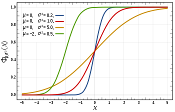
Notation	N(μ,σ2){displaystyle {mathcal {N}}(mu ,sigma ^{2})}
Parameters	; μ∈R{displaystyle mu in mathbb {R} } = mean (location); σ2>0{displaystyle sigma ^{2}>0} = variance (squared scale)
Support	x∈R{displaystyle xin mathbb {R} }
PDF	12πσ2e−(x−μ)22σ2{displaystyle {frac {1}{sqrt {2pi sigma ^{2}}}}e^{-{frac {(x-mu )^{2}}{2sigma ^{2}}}}}
CDF	12[1+erf⁡(x−μσ2)]{displaystyle {frac {1}{2}}left[1+operatorname {erf} left({frac {x-mu }{sigma {sqrt {2}}}}right)right]}
Quantile	μ+σ2erf−1⁡(2F−1){displaystyle mu +sigma {sqrt {2}}operatorname {erf} ^{-1}(2F-1)}
Mean	μ{displaystyle mu }
Median	μ{displaystyle mu }
Mode	μ{displaystyle mu }
Variance	σ2{displaystyle sigma ^{2}}
Skewness	0{displaystyle 0}
Ex. kurtosis	0{displaystyle 0}
Entropy	12log⁡(2πeσ2){displaystyle {frac {1}{2}}log(2pi esigma ^{2})}
MGF	exp⁡(μt+σ2t2/2){displaystyle exp(mu t+sigma ^{2}t^{2}/2)}
CF	exp⁡(iμt−σ2t2/2){displaystyle exp(imu t-sigma ^{2}t^{2}/2)}
Fisher information	; I(μ,σ)=(1/σ2002/σ2){displaystyle {mathcal {I}}(mu ,sigma )={begin{pmatrix}1/sigma ^{2}&0\0&2/sigma ^{2}end{pmatrix}}} ; I(μ,σ2)=(1/σ2001/(2σ4)){displaystyle {mathcal {I}}(mu ,sigma ^{2})={begin{pmatrix}1/sigma ^{2}&0\0&1/(2sigma ^{4})end{pmatrix}}};

In probability theory, the normal (or Gaussian or Gauss or Laplace–Gauss) distribution is a very common continuous probability distribution. Normal distributions are important in statistics and are often used in the natural and social sciences to represent real-valued random variables whose distributions are not known.^[1]^[2] A random variable with a Gaussian distribution is said to be normally distributed and is called a normal deviate.

The normal distribution is useful because of the central limit theorem. In its most general form, under some conditions (which include finite variance), it states that averages of samples of observations of random variables independently drawn from independent distributions converge in distribution to the normal, that is, they become normally distributed when the number of observations is sufficiently large. Physical quantities that are expected to be the sum of many independent processes (such as measurement errors) often have distributions that are nearly normal.^[3] Moreover, many results and methods (such as propagation of uncertainty and least squares parameter fitting) can be derived analytically in explicit form when the relevant variables are normally distributed.

The normal distribution is sometimes informally called the bell curve. However, many other distributions are bell-shaped (such as the Cauchy, Student's t, and logistic distributions).

The probability density of the normal distribution is

{displaystyle f(xmid mu ,sigma ^{2})={frac {1}{sqrt {2pi sigma ^{2}}}}e^{-{frac {(x-mu )^{2}}{2sigma ^{2}}}}}

where

$mu$ is the mean or expectation of the distribution (and also its median and mode),

$sigma$ is the standard deviation, and

$sigma ^{2}$ is the variance.

Definition

Standard normal distribution

The simplest case of a normal distribution is known as the standard normal distribution. This is a special case when $mu =0$ and $sigma =1$ , and it is described by this probability density function:

{displaystyle varphi (x)={frac {1}{sqrt {2pi }}}e^{-{frac {1}{2}}x^{2}}}

The factor $1/{sqrt {2pi }}$ in this expression ensures that the total area under the curve $varphi (x)$ is equal to one.^[4] The factor $1/2$ in the exponent ensures that the distribution has unit variance (i.e. the variance is equal to one), and therefore also unit standard deviation. This function is symmetric around $x=0$ , where it attains its maximum value $1/{sqrt {2pi }}$ and has inflection points at ${displaystyle x=+1}$ and $x=-1$ .

Authors may differ also on which normal distribution should be called the "standard" one. Gauss defined the standard normal as having variance ${displaystyle sigma ^{2}=1/2}$ , that is

{displaystyle varphi (x)={frac {e^{-x^{2}}}{sqrt {pi }}}}

Stigler^[5] goes even further, defining the standard normal with variance ${displaystyle sigma ^{2}=1/(2pi )}$ :

{displaystyle varphi (x)=e^{-pi x^{2}}}

General normal distribution

Every normal distribution is a version of the standard normal distribution whose domain has been stretched by a factor $sigma$ (the standard deviation) and then translated by $mu$ (the mean value):

{displaystyle f(xmid mu ,sigma ^{2})={frac {1}{sigma }}varphi left({frac {x-mu }{sigma }}right).}

The probability density must be scaled by $1/sigma$ so that the integral is still 1.

If $Z$ is a standard normal deviate, then ${displaystyle X=sigma Z+mu }$ will have a normal distribution with expected value $mu$ and standard deviation $sigma$ . Conversely, if $X$ is a normal deviate with parameters $mu$ and $sigma ^{2}$ , then ${displaystyle Z=(X-mu )/sigma }$ will have a standard normal distribution. This variate is called the standardized form of $X$

Every normal distribution is the exponential of a quadratic function:

{displaystyle f(x)=e^{ax^{2}+bx+c}}

where $a<0$ and ${displaystyle c=b^{2}/(4a)+ln(-a/pi )/2}$ . In this form, the mean value is ${displaystyle mu =-b/(2a)}$ , and the variance is ${displaystyle sigma ^{2}=-1/(2a)}$ . For the standard normal distribution, ${displaystyle a=-1/2}$ , $b=0$ , and ${displaystyle c=-ln(2pi )/2}$ .

Notation

The probability density of the standard Gaussian distribution (standard normal distribution) (with zero mean and unit variance) is often denoted with the Greek letter $phi$ (phi).^[6] The alternative form of the Greek letter phi, $varphi$ , is also used quite often.

The normal distribution is often referred to as $N(mu ,sigma ^{2})$ or ${mathcal {N}}(mu ,sigma ^{2})$ .^[7] Thus when a random variable $X$ is distributed normally with mean $mu$ and variance $sigma ^{2}$ , one may write

{displaystyle Xsim {mathcal {N}}(mu ,sigma ^{2}).}

Alternative parameterizations

Some authors advocate using the precision $tau$ as the parameter defining the width of the distribution, instead of the deviation $sigma$ or the variance $sigma ^{2}$ . The precision is normally defined as the reciprocal of the variance, ${displaystyle 1/sigma ^{2}}$ .^[8] The formula for the distribution then becomes

{displaystyle f(x)={sqrt {frac {tau }{2pi }}}e^{-tau (x-mu )^{2}/2}.}

This choice is claimed to have advantages in numerical computations when $sigma$ is very close to zero and simplify formulas in some contexts, such as in the Bayesian inference of variables with multivariate normal distribution.

Also the reciprocal of the standard deviation $tau ^{prime }=1/sigma$ might be defined as the precision and the expression of the normal distribution becomes

{displaystyle f(x)={frac {tau ^{prime }}{sqrt {2pi }}}e^{-(tau ^{prime })^{2}(x-mu )^{2}/2}.}

According to Stigler, this formulation is advantageous because of a much simpler and easier-to-remember formula, and simple approximate formulas for the quantiles of the distribution.

Properties

The normal distribution is the only absolutely continuous distribution whose cumulants beyond the first two (i.e., other than the mean and variance) are zero. It is also the continuous distribution with the maximum entropy for a specified mean and variance.^[9]^[10] Geary has shown, assuming that the mean and variance are finite, that the normal distribution is the only distribution where the mean and variance calculated from a set of independent draws are independent of each other.^[11]^[12]

The normal distribution is a subclass of the elliptical distributions. The normal distribution is symmetric about its mean, and is non-zero over the entire real line. As such it may not be a suitable model for variables that are inherently positive or strongly skewed, such as the weight of a person or the price of a share. Such variables may be better described by other distributions, such as the log-normal distribution or the Pareto distribution.

The value of the normal distribution is practically zero when the value $x$ lies more than a few standard deviations away from the mean (e.g., a spread of three standard deviations covers all but 0.27% of the total distribution). Therefore, it may not be an appropriate model when one expects a significant fraction of outliers—values that lie many standard deviations away from the mean—and least squares and other statistical inference methods that are optimal for normally distributed variables often become highly unreliable when applied to such data. In those cases, a more heavy-tailed distribution should be assumed and the appropriate robust statistical inference methods applied.

The Gaussian distribution belongs to the family of stable distributions which are the attractors of sums of independent, identically distributed distributions whether or not the mean or variance is finite. Except for the Gaussian which is a limiting case, all stable distributions have heavy tails and infinite variance. It is one of the few distributions that are stable and that have probability density functions that can be expressed analytically, the others being the Cauchy distribution and the Lévy distribution.

Symmetries and derivatives

The normal distribution with density $f(x)$ (mean $mu$ and standard deviation $sigma >0$ ) has the following properties:

It is symmetric around the point ${displaystyle x=mu ,}$ which is at the same time the mode, the median and the mean of the distribution.^[13]

It is unimodal: its first derivative is positive for ${displaystyle x<mu ,}$ negative for ${displaystyle x>mu ,}$ and zero only at ${displaystyle x=mu .}$

The area under the curve and over the $x$ -axis is unity (i.e. equal to one).

Its density has two inflection points (where the second derivative of $f$ is zero and changes sign), located one standard deviation away from the mean, namely at ${displaystyle x=mu -sigma }$ and ${displaystyle x=mu +sigma .}$ ^[13]

Its density is log-concave.^[13]

Its density is infinitely differentiable, indeed supersmooth of order 2.^[14]

Furthermore, the density $varphi$ of the standard normal distribution (i.e. $mu =0$ and ${displaystyle sigma =1}$ ) also has the following properties:

Its first derivative is ${displaystyle varphi ^{prime }(x)=-xvarphi (x).}$

Its second derivative is ${displaystyle varphi ^{prime prime }(x)=(x^{2}-1)varphi (x)}$

More generally, its $n$ th derivative is ${displaystyle varphi ^{(n)}(x)=(-1)^{n}operatorname {He} _{n}(x)varphi (x),}$ where ${displaystyle operatorname {He} _{n}(x)}$ is the $n$ th (probabilist) Hermite polynomial.^[15]

The probability that a normally distributed variable $X$ with known $mu$ and $sigma$ is in a particular set, can be calculated by using the fact that the fraction ${displaystyle Z=(X-mu )/sigma }$ has a standard normal distribution.

Moments

The plain and absolute moments of a variable $X$ are the expected values of ${displaystyle X^{p}}$ and ${displaystyle |X|^{p}}$ , respectively. If the expected value $mu$ of $X$ is zero, these parameters are called central moments. Usually we are interested only in moments with integer order $p$ .

If $X$ has a normal distribution, these moments exist and are finite for any $p$ whose real part is greater than −1. For any non-negative integer $p$ , the plain central moments are:^[16]

{displaystyle operatorname {E} left[X^{p}right]={begin{cases}0&{text{if }}p{text{ is odd,}}\sigma ^{p}(p-1)!!&{text{if }}p{text{ is even.}}end{cases}}}

Here $n!!$ denotes the double factorial, that is, the product of all numbers from $n$ to 1 that have the same parity as $n.$

The central absolute moments coincide with plain moments for all even orders, but are nonzero for odd orders. For any non-negative integer $p,$

{displaystyle operatorname {E} left[|X|^{p}right]=sigma ^{p}(p-1)!!cdot left.{begin{cases}{sqrt {frac {2}{pi }}}&{text{if }}p{text{ is odd}}\1&{text{if }}p{text{ is even}}end{cases}}right}=sigma ^{p}cdot {frac {2^{p/2}Gamma left({frac {p+1}{2}}right)}{sqrt {pi }}}}

The last formula is valid also for any non-integer ${displaystyle p>-1.}$ When the mean ${displaystyle mu neq 0,}$ the plain and absolute moments can be expressed in terms of confluent hypergeometric functions ${}_{1}F_{1}$ and $U.$ ^{[citation needed]}

{displaystyle operatorname {E} left[X^{p}right]=sigma ^{p}cdot (-i{sqrt {2}})^{p}Uleft(-{frac {p}{2}},{frac {1}{2}},-{frac {1}{2}}left({frac {mu }{sigma }}right)^{2}right),}

{displaystyle operatorname {E} left[|X|^{p}right]=sigma ^{p}cdot 2^{p/2}{frac {Gamma left({frac {1+p}{2}}right)}{sqrt {pi }}}{}_{1}F_{1}left(-{frac {p}{2}},{frac {1}{2}},-{frac {1}{2}}left({frac {mu }{sigma }}right)^{2}right).}

These expressions remain valid even if $p$ is not integer. See also generalized Hermite polynomials.

Order	Non-central moment	Central moment
1	$mu$	${displaystyle 0}$
2	${displaystyle mu ^{2}+sigma ^{2}}$	$sigma ^{2}$
3	${displaystyle mu ^{3}+3mu sigma ^{2}}$	${displaystyle 0}$
4	${displaystyle mu ^{4}+6mu ^{2}sigma ^{2}+3sigma ^{4}}$	${displaystyle 3sigma ^{4}}$
5	${displaystyle mu ^{5}+10mu ^{3}sigma ^{2}+15mu sigma ^{4}}$	${displaystyle 0}$
6	${displaystyle mu ^{6}+15mu ^{4}sigma ^{2}+45mu ^{2}sigma ^{4}+15sigma ^{6}}$	${displaystyle 15sigma ^{6}}$
7	${displaystyle mu ^{7}+21mu ^{5}sigma ^{2}+105mu ^{3}sigma ^{4}+105mu sigma ^{6}}$	${displaystyle 0}$
8	${displaystyle mu ^{8}+28mu ^{6}sigma ^{2}+210mu ^{4}sigma ^{4}+420mu ^{2}sigma ^{6}+105sigma ^{8}}$	${displaystyle 105sigma ^{8}}$

The expectation of $X$ conditioned on the event that $X$ lies in an interval $[a,b]$ is given by

{displaystyle operatorname {E} left[Xmid a<X<bright]=mu -sigma ^{2}{frac {f(b)-f(a)}{F(b)-F(a)}}}

where $f$ and $F$ respectively are the density and the cumulative distribution function of $X$ . For $b=infty$ this is known as the inverse Mills ratio. Note that above, density $f$ of $X$ is used instead of standard normal density as in inverse Mills ratio, so here we have $sigma ^{2}$ instead of $sigma$ .

Fourier transform and characteristic function

The Fourier transform of a normal density $f$ with mean $mu$ and standard deviation $sigma$ is^[17]

{displaystyle {hat {f}}(t)=int _{-infty }^{infty }f(x)e^{-itx},dx=e^{-imu t}e^{-{frac {1}{2}}(sigma t)^{2}}}

where $i$ is the imaginary unit. If the mean $mu =0$ , the first factor is 1, and the Fourier transform is, apart from a constant factor, a normal density on the frequency domain, with mean 0 and standard deviation $1/sigma$ . In particular, the standard normal distribution $varphi$ is an eigenfunction of the Fourier transform.

In probability theory, the Fourier transform of the probability distribution of a real-valued random variable $X$ is closely connected to the characteristic function $varphi _{X}(t)$ of that variable, which is defined as the expected value of $e^{{itX}}$ , as a function of the real variable $t$ (the frequency parameter of the Fourier transform). This definition can be analytically extended to a complex-value variable $t$ .^[18] The relation between both is:

{displaystyle varphi _{X}(t)={hat {f}}(-t)}

Moment and cumulant generating functions

The moment generating function of a real random variable $X$ is the expected value of ${displaystyle e^{tX}}$ , as a function of the real parameter $t$ . For a normal distribution with density $f$ , mean $mu$ and deviation $sigma$ , the moment generating function exists and is equal to

{displaystyle M(t)=operatorname {E} [e^{tX}]={hat {f}}(it)=e^{mu t}e^{{tfrac {1}{2}}sigma ^{2}t^{2}}}

The cumulant generating function is the logarithm of the moment generating function, namely

{displaystyle g(t)=ln M(t)=mu t+{tfrac {1}{2}}sigma ^{2}t^{2}}

Since this is a quadratic polynomial in $t$ , only the first two cumulants are nonzero, namely the mean $mu$ and the variance $sigma ^{2}$ .

Cumulative distribution function

The cumulative distribution function (CDF) of the standard normal distribution, usually denoted with the capital Greek letter $Phi$ (phi), is the integral

{displaystyle Phi (x)={frac {1}{sqrt {2pi }}}int _{-infty }^{x}e^{-t^{2}/2},dt}

The related error function $operatorname{erf}(x)$ gives the probability of a random variable with normal distribution of mean 0 and variance 1/2 falling in the range $[-x,x]$ ; that is

{displaystyle operatorname {erf} (x)={frac {2}{sqrt {pi }}}int _{0}^{x}e^{-t^{2}},dt}

These integrals cannot be expressed in terms of elementary functions, and are often said to be special functions. However, many numerical approximations are known; see below.

The two functions are closely related, namely

{displaystyle Phi (x)={frac {1}{2}}left[1+operatorname {erf} left({frac {x}{sqrt {2}}}right)right]}

For a generic normal distribution with density $f$ , mean $mu$ and deviation $sigma$ , the cumulative distribution function is

{displaystyle F(x)=Phi left({frac {x-mu }{sigma }}right)={frac {1}{2}}left[1+operatorname {erf} left({frac {x-mu }{sigma {sqrt {2}}}}right)right]}

The complement of the standard normal CDF, $Q(x)=1-Phi (x)$ , is often called the Q-function, especially in engineering texts.^[19]^[20] It gives the probability that the value of a standard normal random variable $X$ will exceed $x$ : ${displaystyle P(X>x)}$ . Other definitions of the $Q$ -function, all of which are simple transformations of $Phi$ , are also used occasionally.^[21]

The graph of the standard normal CDF $Phi$ has 2-fold rotational symmetry around the point (0,1/2); that is, $Phi (-x)=1-Phi (x)$ . Its antiderivative (indefinite integral) is

{displaystyle int Phi (x),dx=xPhi (x)+varphi (x)+C.}

The CDF of the standard normal distribution can be expanded by Integration by parts into a series:

{displaystyle Phi (x)={frac {1}{2}}+{frac {1}{sqrt {2pi }}}cdot e^{-x^{2}/2}left[x+{frac {x^{3}}{3}}+{frac {x^{5}}{3cdot 5}}+cdots +{frac {x^{2n+1}}{(2n+1)!!}}+cdots right]}

where $!!$ denotes the double factorial.

An asymptotic expansion of the CDF for large x can also be derived using integration by parts; see Error function#Asymptotic expansion.^[22]

Standard deviation and coverage

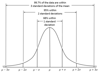
For the normal distribution, the values less than one standard deviation away from the mean account for 68.27% of the set; while two standard deviations from the mean account for 95.45%; and three standard deviations account for 99.73%.

About 68% of values drawn from a normal distribution are within one standard deviation σ away from the mean; about 95% of the values lie within two standard deviations; and about 99.7% are within three standard deviations. This fact is known as the 68-95-99.7 (empirical) rule, or the 3-sigma rule.

More precisely, the probability that a normal deviate lies in the range between ${displaystyle mu -nsigma }$ and ${displaystyle mu +nsigma }$ is given by

{displaystyle F(mu +nsigma )-F(mu -nsigma )=Phi (n)-Phi (-n)=operatorname {erf} left({frac {n}{sqrt {2}}}right).}

To 12 significant figures, the values for ${displaystyle n=1,2,ldots ,6}$ are:^[23]

n

{displaystyle p=F(mu +nsigma )-F(mu -nsigma )}

{displaystyle {text{i.e. }}1-p}

{displaystyle {text{or }}1{text{ in }}p}

OEIS

1

6999682689492137000♠0.682689492137

6999317310507863000♠0.317310507863

7000300000000000000♠3

.15148718753

OEIS: A178647

2

6999954499736104000♠0.954499736104

6998455002638960000♠0.045500263896

7001210000000000000♠21

.9778945080

OEIS: A110894

3

6999997300203937000♠0.997300203937

6997269979606300000♠0.002699796063

7002370000000000000♠370

.398347345

OEIS: A270712

4

6999999936657516000♠0.999936657516

6995633424840000000♠0.000063342484

7004157870000000000♠15787

.1927673

5

6999999999426697000♠0.999999426697

6993573303000000000♠0.000000573303

7006174427700000000♠1744277

.89362

6

6999999999998027000♠0.999999998027

6991197300000000000♠0.000000001973

7008506797345000000♠506797345

.897

Quantile function

The quantile function of a distribution is the inverse of the cumulative distribution function. The quantile function of the standard normal distribution is called the probit function, and can be expressed in terms of the inverse error function:

{displaystyle Phi ^{-1}(p)={sqrt {2}}operatorname {erf} ^{-1}(2p-1),quad pin (0,1).}

For a normal random variable with mean $mu$ and variance $sigma ^{2}$ , the quantile function is

{displaystyle F^{-1}(p)=mu +sigma Phi ^{-1}(p)=mu +sigma {sqrt {2}}operatorname {erf} ^{-1}(2p-1),quad pin (0,1).}

The quantile $Phi ^{{-1}}(p)$ of the standard normal distribution is commonly denoted as ${displaystyle z_{p}}$ . These values are used in hypothesis testing, construction of confidence intervals and Q-Q plots. A normal random variable $X$ will exceed ${displaystyle mu +z_{p}sigma }$ with probability $1-p$ , and will lie outside the interval ${displaystyle mu pm z_{p}sigma }$ with probability ${displaystyle 2(1-p)}$ . In particular, the quantile ${displaystyle z_{0.975}}$ is 1.96; therefore a normal random variable will lie outside the interval $mu pm 1.96sigma$ in only 5% of cases.

The following table gives the quantile ${displaystyle z_{p}}$ such that $X$ will lie in the range ${displaystyle mu pm z_{p}sigma }$ with a specified probability $p$ . These values are useful to determine tolerance interval for sample averages and other statistical estimators with normal (or asymptotically normal) distributions:.^[24]^[25] NOTE: the following table shows ${displaystyle {sqrt {2}}operatorname {erf} ^{-1}(p)=Phi ^{-1}left({frac {p+1}{2}}right)}$ , not $Phi ^{{-1}}(p)$ as defined above.

$p$	${displaystyle z_{p}}$	$p$	${displaystyle z_{p}}$
0.80	7000128155156554500♠1.281551565545	0.999	7000329052673149200♠3.290526731492
0.90	7000164485362695100♠1.644853626951	0.9999	7000389059188641300♠3.890591886413
0.95	7000195996398454000♠1.959963984540	0.99999	7000441717341346900♠4.417173413469
0.98	7000232634787404100♠2.326347874041	0.999999	7000489163847569899♠4.891638475699
0.99	7000257582930354900♠2.575829303549	0.9999999	7000532672388638400♠5.326723886384
0.995	7000280703376834400♠2.807033768344	0.99999999	7000573072886823600♠5.730728868236
0.998	7000309023230616800♠3.090232306168	0.999999999	7000610941020486900♠6.109410204869

For small $p$ , the quantile function has the useful asymptotic expansion
${displaystyle Phi ^{-1}(p)=-{sqrt {ln {frac {1}{p^{2}}}-ln ln {frac {1}{p^{2}}}-ln(2pi )}}+{mathcal {o}}(1).}$

Zero-variance limit

In the limit when $sigma$ tends to zero, the probability density $f(x)$ eventually tends to zero at any ${displaystyle xneq mu }$ , but grows without limit if ${displaystyle x=mu }$ , while its integral remains equal to 1. Therefore, the normal distribution cannot be defined as an ordinary function when $sigma =0$ .

However, one can define the normal distribution with zero variance as a generalized function; specifically, as Dirac's "delta function" $delta$ translated by the mean $mu$ , that is ${displaystyle f(x)=delta (x-mu ).}$
Its CDF is then the Heaviside step function translated by the mean $mu$ , namely

{displaystyle F(x)={begin{cases}0&{text{if }}x<mu \1&{text{if }}xgeq mu end{cases}}}

Central limit theorem

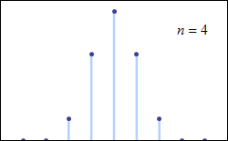
As the number of discrete events increases, the function begins to resemble a normal distribution

Comparison of probability density functions,

p(k)

for the sum of

n

fair 6-sided dice to show their convergence to a normal distribution with increasing

{displaystyle na}

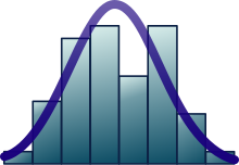
, in accordance to the central limit theorem. In the bottom-right graph, smoothed profiles of the previous graphs are rescaled, superimposed and compared with a normal distribution (black curve).

The central limit theorem states that under certain (fairly common) conditions, the sum of many random variables will have an approximately normal distribution. More specifically, where ${displaystyle X_{1},ldots ,X_{n}}$ are independent and identically distributed random variables with the same arbitrary distribution, zero mean, and variance $sigma ^{2}$ and $Z$ is their
mean scaled by ${sqrt {n}}$

Z={sqrt {n}}left({frac {1}{n}}sum _{i=1}^{n}X_{i}right)

Then, as $n$ increases, the probability distribution of $Z$ will tend to the normal distribution with zero mean and variance $sigma ^{2}$ .

The theorem can be extended to variables $(X_{i})$ that are not independent and/or not identically distributed if certain constraints are placed on the degree of dependence and the moments of the distributions.

Many test statistics, scores, and estimators encountered in practice contain sums of certain random variables in them, and even more estimators can be represented as sums of random variables through the use of influence functions. The central limit theorem implies that those statistical parameters will have asymptotically normal distributions.

The central limit theorem also implies that certain distributions can be approximated by the normal distribution, for example:

The binomial distribution $B(n,p)$ is approximately normal with mean $np$ and variance $np(1-p)$ for large $n$ and for $p$ not too close to 0 or 1.

The Poisson distribution with parameter $lambda$ is approximately normal with mean $lambda$ and variance $lambda$ , for large values of $lambda$ .^[26]

The chi-squared distribution ${displaystyle chi ^{2}(k)}$ is approximately normal with mean $k$ and variance $2k$ , for large $k$ .

The Student's t-distribution ${displaystyle t(nu )}$ is approximately normal with mean 0 and variance 1 when $nu$ is large.

Whether these approximations are sufficiently accurate depends on the purpose for which they are needed, and the rate of convergence to the normal distribution. It is typically the case that such approximations are less accurate in the tails of the distribution.

A general upper bound for the approximation error in the central limit theorem is given by the Berry–Esseen theorem, improvements of the approximation are given by the Edgeworth expansions.

Maximum entropy

Of all probability distributions over the reals with a specified mean $mu$ and variance $sigma ^{2}$ , the normal distribution $N(mu ,sigma ^{2})$ is the one with maximum entropy.^[27] If $X$ is a continuous random variable with probability density $f(x)$ , then the entropy of $X$ is defined as^[28]^[29]^[30]

{displaystyle H(X)=-int _{-infty }^{infty }f(x)log f(x),dx={tfrac {1}{2}}(1+log(2sigma ^{2}pi ))}

where ${displaystyle f(x)log f(x)}$ is understood to be zero whenever $f(x)=0$ . This functional can be maximized, subject to the constraints that the distribution is properly normalized and has a specified variance, by using variational calculus. A function with two Lagrange multipliers is defined:

{displaystyle L=int _{-infty }^{infty }f(x)ln(f(x)),dx-lambda _{0}left(1-int _{-infty }^{infty }f(x),dxright)-lambda left(sigma ^{2}-int _{-infty }^{infty }f(x)(x-mu )^{2},dxright)}

where $f(x)$ is, for now, regarded as some density function with mean $mu$ and standard deviation $sigma$ .

At maximum entropy, a small variation ${displaystyle delta f(x)}$ about $f(x)$ will produce a variation $delta L$ about $L$ which is equal to 0:

{displaystyle 0=delta L=int _{-infty }^{infty }delta f(x)left(ln(f(x))+1+lambda _{0}+lambda (x-mu )^{2}right),dx}

Since this must hold for any small ${displaystyle delta f(x)}$ , the term in brackets must be zero, and solving for $f(x)$ yields:

f(x)=e^{-lambda _{0}-1-lambda (x-mu )^{2}}

Using the constraint equations to solve for $lambda _{0}$ and $lambda$ yields the density of the normal distribution:

{displaystyle f(x,mu ,sigma )={frac {1}{sqrt {2pi sigma ^{2}}}}e^{-{frac {(x-mu )^{2}}{2sigma ^{2}}}}}

Operations on normal deviates

The family of normal distributions is closed under linear transformations: if X is normally distributed with mean μ and standard deviation σ, then the variable Y = aX + b, for any real numbers a and b, is also normally distributed, with
mean aμ + b and standard deviation |a|σ.

Also if X₁ and X₂ are two independent normal random variables, with means μ₁, μ₂ and standard deviations σ₁, σ₂, then their sum X₁ + X₂ will also be normally distributed,^[proof] with mean μ₁ + μ₂ and variance $sigma _{1}^{2}+sigma _{2}^{2}$ .

In particular, if X and Y are independent normal deviates with zero mean and variance σ², then X + Y and X − Y are also independent and normally distributed, with zero mean and variance 2σ². This is a special case of the polarization identity.^[31]

Also, if X₁, X₂ are two independent normal deviates with mean μ and deviation σ, and a, b are arbitrary real numbers, then the variable

X_{3}={frac {aX_{1}+bX_{2}-(a+b)mu }{sqrt {a^{2}+b^{2}}}}+mu

is also normally distributed with mean μ and deviation σ. It follows that the normal distribution is stable (with exponent α = 2).

More generally, any linear combination of independent normal deviates is a normal deviate.

Infinite divisibility and Cramér's theorem

For any positive integer n, any normal distribution with mean μ and variance σ² is the distribution of the sum of n independent normal deviates, each with mean μ/n and variance σ²/n. This property is called infinite divisibility.^[32]

Conversely, if X₁ and X₂ are independent random variables and their sum X₁ + X₂ has a normal distribution, then both X₁ and X₂ must be normal deviates.^[33]

This result is known as Cramér's decomposition theorem, and is equivalent to saying that the convolution of two distributions is normal if and only if both are normal. Cramér's theorem implies that a linear combination of independent non-Gaussian variables will never have an exactly normal distribution, although it may approach it arbitrarily closely.^[34]

Bernstein's theorem

Bernstein's theorem states that if X and Y are independent and X + Y and X − Y are also independent, then both X and Y must necessarily have normal distributions.^[35]^[36]

More generally, if X₁, …, X_n are independent random variables, then two distinct linear combinations ∑a_kX_k and ∑b_kX_k will be independent if and only if all X_k's are normal and ∑a_kb_kσ 2
k = 0, where σ 2
k denotes the variance of X_k.^[35]

Other properties

If the characteristic function φ_X of some random variable X is of the form φ_X(t) = e^Q(t), where Q(t) is a polynomial, then the Marcinkiewicz theorem (named after Józef Marcinkiewicz) asserts that Q can be at most a quadratic polynomial, and therefore X is a normal random variable.^[34] The consequence of this result is that the normal distribution is the only distribution with a finite number (two) of non-zero cumulants.

If X and Y are jointly normal and uncorrelated, then they are independent. The requirement that X and Y should be jointly normal is essential; without it the property does not hold.^[37]^[38]^[proof] For non-normal random variables uncorrelatedness does not imply independence.

The Kullback–Leibler divergence of one normal distribution X₁ ∼ N(μ₁, σ²₁ )from another X₂ ∼ N(μ₂, σ²₂ )is given by:^[39]
${displaystyle D_{mathrm {KL} }(X_{1},|,X_{2})={frac {(mu _{1}-mu _{2})^{2}}{2sigma _{2}^{2}}}+{frac {1}{2}}left({frac {sigma _{1}^{2}}{sigma _{2}^{2}}}-1-ln {frac {sigma _{1}^{2}}{sigma _{2}^{2}}}right).}$

The Hellinger distance between the same distributions is equal to

${displaystyle H^{2}(X_{1},X_{2})=1-{sqrt {frac {2sigma _{1}sigma _{2}}{sigma _{1}^{2}+sigma _{2}^{2}}}}e^{-{frac {1}{4}}{frac {(mu _{1}-mu _{2})^{2}}{sigma _{1}^{2}+sigma _{2}^{2}}}}.}$

The Fisher information matrix for a normal distribution is diagonal and takes the form

${mathcal {I}}={begin{pmatrix}{frac {1}{sigma ^{2}}}&0\0&{frac {1}{2sigma ^{4}}}end{pmatrix}}$

Normal distributions belong to an exponential family with natural parameters ${displaystyle textstyle theta _{1}={frac {mu }{sigma ^{2}}}}$ and ${displaystyle textstyle theta _{2}={frac {-1}{2sigma ^{2}}}}$ , and natural statistics x and x². The dual, expectation parameters for normal distribution are η₁ = μ and η₂ = μ² + σ².

The conjugate prior of the mean of a normal distribution is another normal distribution.^[40] Specifically, if x₁, …, x_n are iid N(μ, σ²) and the prior is μ ~ N(μ₀, σ²
₀), then the posterior distribution for the estimator of μ will be

${displaystyle mu mid x_{1},ldots ,x_{n}sim {mathcal {N}}left({frac {{frac {sigma ^{2}}{n}}mu _{0}+sigma _{0}^{2}{bar {x}}}{{frac {sigma ^{2}}{n}}+sigma _{0}^{2}}},left({frac {n}{sigma ^{2}}}+{frac {1}{sigma _{0}^{2}}}right)^{-1}right)}$

The family of normal distributions forms a manifold with constant curvature −1. The same family is flat with respect to the (±1)-connections ∇^(e) and ∇^(m).^[41]

Related distributions

Operations on a single random variable

If X is distributed normally with mean μ and variance σ², then

The exponential of X is distributed log-normally: e^X ~ ln(N (μ, σ²)).

The absolute value of X has folded normal distribution: |X| ~ N_f (μ, σ²). If μ = 0 this is known as the half-normal distribution.

The absolute value of normalized residuals, |X − μ|/σ, has chi distribution with one degree of freedom: |X − μ|/σ ~ χ₁(|X − μ|/σ).

The square of X/σ has the noncentral chi-squared distribution with one degree of freedom: X²/σ² ~ χ²₁(μ²/σ²). If μ = 0, the distribution is called simply chi-squared.

The distribution of the variable X restricted to an interval [a, b] is called the truncated normal distribution.

(X − μ)⁻² has a Lévy distribution with location 0 and scale σ⁻².

Combination of two independent random variables

If X₁ and X₂ are two independent standard normal random variables with mean 0 and variance 1, then

Their sum and difference is distributed normally with mean zero and variance two: X₁ ± X₂ ∼ N(0, 2).

Their product Z = X₁·X₂ follows the "product-normal" distribution^[42] with density function f_Z(z) = $π$ ⁻¹K₀(|z|), where K₀ is the modified Bessel function of the second kind. This distribution is symmetric around zero, unbounded at z = 0, and has the characteristic function φ_Z(t) = (1 + t²)^−1/2.

Their ratio follows the standard Cauchy distribution: X₁ / X₂ ∼ Cauchy(0, 1).

Their Euclidean norm ${displaystyle {sqrt {X_{1}^{2}+X_{2}^{2}}}}$ has the Rayleigh distribution.

Combination of two or more independent random variables

If X₁, X₂, …, X_n are independent standard normal random variables, then the sum of their squares has the chi-squared distribution with n degrees of freedom

{displaystyle X_{1}^{2}+cdots +X_{n}^{2}sim chi _{n}^{2}.}

If X₁, X₂, …, X_n are independent normally distributed random variables with means μ and variances σ², then their sample mean is independent from the sample standard deviation,^[43] which can be demonstrated using Basu's theorem or Cochran's theorem.^[44] The ratio of these two quantities will have the Student's t-distribution with n − 1 degrees of freedom:

{displaystyle t={frac {{overline {X}}-mu }{S/{sqrt {n}}}}={frac {{frac {1}{n}}(X_{1}+cdots +X_{n})-mu }{sqrt {{frac {1}{n(n-1)}}left[(X_{1}-{overline {X}})^{2}+cdots +(X_{n}-{overline {X}})^{2}right]}}}sim t_{n-1}.}

' If X₁, …, X_n, Y₁, …, Y_m are independent standard normal random variables, then the ratio of their normalized sums of squares will have the F-distribution with (n, m) degrees of freedom:^[45]

{displaystyle F={frac {left(X_{1}^{2}+X_{2}^{2}+cdots +X_{n}^{2}right)/n}{left(Y_{1}^{2}+Y_{2}^{2}+cdots +Y_{m}^{2}right)/m}}sim F_{n,m}.}

Operations on the density function

The split normal distribution is most directly defined in terms of joining scaled sections of the density functions of different normal distributions and rescaling the density to integrate to one. The truncated normal distribution results from rescaling a section of a single density function.

Extensions

The notion of normal distribution, being one of the most important distributions in probability theory, has been extended far beyond the standard framework of the univariate (that is one-dimensional) case (Case 1). All these extensions are also called normal or Gaussian laws, so a certain ambiguity in names exists.

The multivariate normal distribution describes the Gaussian law in the k-dimensional Euclidean space. A vector X ∈ R^k is multivariate-normally distributed if any linear combination of its components ∑^k
_j=1a_j X_j has a (univariate) normal distribution. The variance of X is a k×k symmetric positive-definite matrix V. The multivariate normal distribution is a special case of the elliptical distributions. As such, its iso-density loci in the k = 2 case are ellipses and in the case of arbitrary k are ellipsoids.

Rectified Gaussian distribution a rectified version of normal distribution with all the negative elements reset to 0

Complex normal distribution deals with the complex normal vectors. A complex vector X ∈ C^k is said to be normal if both its real and imaginary components jointly possess a 2k-dimensional multivariate normal distribution. The variance-covariance structure of X is described by two matrices: the variance matrix Γ, and the relation matrix C.

Matrix normal distribution describes the case of normally distributed matrices.

Gaussian processes are the normally distributed stochastic processes. These can be viewed as elements of some infinite-dimensional Hilbert space H, and thus are the analogues of multivariate normal vectors for the case k = ∞. A random element h ∈ H is said to be normal if for any constant a ∈ H the scalar product (a, h) has a (univariate) normal distribution. The variance structure of such Gaussian random element can be described in terms of the linear covariance operator K: H → H. Several Gaussian processes became popular enough to have their own names:
- Brownian motion,
- Brownian bridge,
- Ornstein–Uhlenbeck process.

Gaussian q-distribution is an abstract mathematical construction that represents a "q-analogue" of the normal distribution.

the q-Gaussian is an analogue of the Gaussian distribution, in the sense that it maximises the Tsallis entropy, and is one type of Tsallis distribution. Note that this distribution is different from the Gaussian q-distribution above.

A random variable X has a two-piece normal distribution if it has a distribution

{displaystyle f_{X}(x)=N(mu ,sigma _{1}^{2}){text{ if }}xleq mu }

{displaystyle f_{X}(x)=N(mu ,sigma _{2}^{2}){text{ if }}xgeq mu }

where μ is the mean and σ₁ and σ₂ are the standard deviations of the distribution to the left and right of the mean respectively.

The mean, variance and third central moment of this distribution have been determined^[46]

{displaystyle operatorname {E} (X)=mu +{sqrt {frac {2}{pi }}}(sigma _{2}-sigma _{1})}

{displaystyle operatorname {V} (X)=left(1-{frac {2}{pi }}right)(sigma _{2}-sigma _{1})^{2}+sigma _{1}sigma _{2}}

{displaystyle operatorname {T} (X)={sqrt {frac {2}{pi }}}(sigma _{2}-sigma _{1})left[left({frac {4}{pi }}-1right)(sigma _{2}-sigma _{1})^{2}+sigma _{1}sigma _{2}right]}

where E(X), V(X) and T(X) are the mean, variance, and third central moment respectively.

One of the main practical uses of the Gaussian law is to model the empirical distributions of many different random variables encountered in practice. In such case a possible extension would be a richer family of distributions, having more than two parameters and therefore being able to fit the empirical distribution more accurately. The examples of such extensions are:

Pearson distribution — a four-parameter family of probability distributions that extend the normal law to include different skewness and kurtosis values.

The generalized normal distribution, also known as the exponential power distribution, allows for distribution tails with thicker or thinner asymptotic behaviors.

Normality tests

Normality tests assess the likelihood that the given data set {x₁, …, x_n} comes from a normal distribution. Typically the null hypothesis H₀ is that the observations are distributed normally with unspecified mean μ and variance σ², versus the alternative H_a that the distribution is arbitrary. Many tests (over 40) have been devised for this problem, the more prominent of them are outlined below:

"Visual" tests are more intuitively appealing but subjective at the same time, as they rely on informal human judgement to accept or reject the null hypothesis.
- Q-Q plot— is a plot of the sorted values from the data set against the expected values of the corresponding quantiles from the standard normal distribution. That is, it's a plot of point of the form (Φ⁻¹(p_k), x_(k)), where plotting points p_k are equal to p_k = (k − α)/(n + 1 − 2α) and α is an adjustment constant, which can be anything between 0 and 1. If the null hypothesis is true, the plotted points should approximately lie on a straight line.
- P-P plot— similar to the Q-Q plot, but used much less frequently. This method consists of plotting the points (Φ(z_(k)), p_k), where ${displaystyle textstyle z_{(k)}=(x_{(k)}-{hat {mu }})/{hat {sigma }}}$ . For normally distributed data this plot should lie on a 45° line between (0, 0) and (1, 1).
- Shapiro-Wilk test employs the fact that the line in the Q-Q plot has the slope of σ. The test compares the least squares estimate of that slope with the value of the sample variance, and rejects the null hypothesis if these two quantities differ significantly.
- Normal probability plot (rankit plot)

Moment tests:
- D'Agostino's K-squared test
- Jarque–Bera test

Empirical distribution function tests:
- Lilliefors test (an adaptation of the Kolmogorov–Smirnov test)
- Anderson–Darling test

Estimation of parameters

It is often the case that we don't know the parameters of the normal distribution, but instead want to estimate them. That is, having a sample (x₁, …, x_n) from a normal N(μ, σ²) population we would like to learn the approximate values of parameters μ and σ². The standard approach to this problem is the maximum likelihood method, which requires maximization of the log-likelihood function:

{displaystyle ln {mathcal {L}}(mu ,sigma ^{2})=sum _{i=1}^{n}ln f(x_{i}mid mu ,sigma ^{2})=-{frac {n}{2}}ln(2pi )-{frac {n}{2}}ln sigma ^{2}-{frac {1}{2sigma ^{2}}}sum _{i=1}^{n}(x_{i}-mu )^{2}.}

Taking derivatives with respect to μ and σ² and solving the resulting system of first order conditions yields the maximum likelihood estimates:

{hat {mu }}={overline {x}}equiv {frac {1}{n}}sum _{i=1}^{n}x_{i},qquad {hat {sigma }}^{2}={frac {1}{n}}sum _{i=1}^{n}(x_{i}-{overline {x}})^{2}.

Sample mean

Estimator ${displaystyle textstyle {hat {mu }}}$ is called the sample mean, since it is the arithmetic mean of all observations. The statistic ${displaystyle textstyle {overline {x}}}$ is complete and sufficient for μ, and therefore by the Lehmann–Scheffé theorem, ${displaystyle textstyle {hat {mu }}}$ is the uniformly minimum variance unbiased (UMVU) estimator.^[47] In finite samples it is distributed normally:

{displaystyle {hat {mu }}sim {mathcal {N}}(mu ,sigma ^{2}/n).}

The variance of this estimator is equal to the μμ-element of the inverse Fisher information matrix ${displaystyle textstyle {mathcal {I}}^{-1}}$ . This implies that the estimator is finite-sample efficient. Of practical importance is the fact that the standard error of ${displaystyle textstyle {hat {mu }}}$ is proportional to ${displaystyle textstyle 1/{sqrt {n}}}$ , that is, if one wishes to decrease the standard error by a factor of 10, one must increase the number of points in the sample by a factor of 100. This fact is widely used in determining sample sizes for opinion polls and the number of trials in Monte Carlo simulations.

From the standpoint of the asymptotic theory, ${displaystyle textstyle {hat {mu }}}$ is consistent, that is, it converges in probability to μ as n → ∞. The estimator is also asymptotically normal, which is a simple corollary of the fact that it is normal in finite samples:

{displaystyle {sqrt {n}}({hat {mu }}-mu ),{xrightarrow {d}},{mathcal {N}}(0,sigma ^{2}).}

Sample variance

The estimator ${displaystyle textstyle {hat {sigma }}^{2}}$ is called the sample variance, since it is the variance of the sample (x₁, …, x_n). In practice, another estimator is often used instead of the ${displaystyle textstyle {hat {sigma }}^{2}}$ . This other estimator is denoted s², and is also called the sample variance, which represents a certain ambiguity in terminology; its square root s is called the sample standard deviation. The estimator s² differs from ${displaystyle textstyle {hat {sigma }}^{2}}$ by having (n − 1) instead of n in the denominator (the so-called Bessel's correction):

{displaystyle s^{2}={frac {n}{n-1}}{hat {sigma }}^{2}={frac {1}{n-1}}sum _{i=1}^{n}(x_{i}-{overline {x}})^{2}.}

The difference between s² and ${displaystyle textstyle {hat {sigma }}^{2}}$ becomes negligibly small for large n's. In finite samples however, the motivation behind the use of s² is that it is an unbiased estimator of the underlying parameter σ², whereas ${displaystyle textstyle {hat {sigma }}^{2}}$ is biased. Also, by the Lehmann–Scheffé theorem the estimator s² is uniformly minimum variance unbiased (UMVU),^[47] which makes it the "best" estimator among all unbiased ones. However it can be shown that the biased estimator ${displaystyle textstyle {hat {sigma }}^{2}}$ is "better" than the s² in terms of the mean squared error (MSE) criterion. In finite samples both s² and ${displaystyle textstyle {hat {sigma }}^{2}}$ have scaled chi-squared distribution with (n − 1) degrees of freedom:

{displaystyle s^{2}sim {frac {sigma ^{2}}{n-1}}cdot chi _{n-1}^{2},qquad {hat {sigma }}^{2}sim {frac {sigma ^{2}}{n}}cdot chi _{n-1}^{2}.}

The first of these expressions shows that the variance of s² is equal to 2σ⁴/(n−1), which is slightly greater than the σσ-element of the inverse Fisher information matrix ${displaystyle textstyle {mathcal {I}}^{-1}}$ . Thus, s² is not an efficient estimator for σ², and moreover, since s² is UMVU, we can conclude that the finite-sample efficient estimator for σ² does not exist.

Applying the asymptotic theory, both estimators s² and ${displaystyle textstyle {hat {sigma }}^{2}}$ are consistent, that is they converge in probability to σ² as the sample size n → ∞. The two estimators are also both asymptotically normal:

{displaystyle {sqrt {n}}({hat {sigma }}^{2}-sigma ^{2})simeq {sqrt {n}}(s^{2}-sigma ^{2}),{xrightarrow {d}},{mathcal {N}}(0,2sigma ^{4}).}

In particular, both estimators are asymptotically efficient for σ².

Confidence intervals

By Cochran's theorem, for normal distributions the sample mean ${displaystyle textstyle {hat {mu }}}$ and the sample variance s² are independent, which means there can be no gain in considering their joint distribution. There is also a converse theorem: if in a sample the sample mean and sample variance are independent, then the sample must have come from the normal distribution. The independence between ${displaystyle textstyle {hat {mu }}}$ and s can be employed to construct the so-called t-statistic:

{displaystyle t={frac {{hat {mu }}-mu }{s/{sqrt {n}}}}={frac {{overline {x}}-mu }{sqrt {{frac {1}{n(n-1)}}sum (x_{i}-{overline {x}})^{2}}}}sim t_{n-1}}

This quantity t has the Student's t-distribution with (n − 1) degrees of freedom, and it is an ancillary statistic (independent of the value of the parameters). Inverting the distribution of this t-statistics will allow us to construct the confidence interval for μ;^[48] similarly, inverting the χ² distribution of the statistic s² will give us the confidence interval for σ²:^[49]

{displaystyle mu in left[{hat {mu }}-t_{n-1,1-alpha /2}{frac {1}{sqrt {n}}}s,{hat {mu }}+t_{n-1,1-alpha /2}{frac {1}{sqrt {n}}}sright]approx left[{hat {mu }}-|z_{alpha /2}|{frac {1}{sqrt {n}}}s,{hat {mu }}+|z_{alpha /2}|{frac {1}{sqrt {n}}}sright],}

{displaystyle sigma ^{2}in left[{frac {(n-1)s^{2}}{chi _{n-1,1-alpha /2}^{2}}},{frac {(n-1)s^{2}}{chi _{n-1,alpha /2}^{2}}}right]approx left[s^{2}-|z_{alpha /2}|{frac {sqrt {2}}{sqrt {n}}}s^{2},s^{2}+|z_{alpha /2}|{frac {sqrt {2}}{sqrt {n}}}s^{2}right],}

where t_k,p and χ 2
k,p are the pth quantiles of the t- and χ²-distributions respectively. These confidence intervals are of the confidence level 1 − α, meaning that the true values μ and σ² fall outside of these intervals with probability (or significance level) α. In practice people usually take α = 5%, resulting in the 95% confidence intervals. The approximate formulas in the display above were derived from the asymptotic distributions of ${displaystyle textstyle {hat {mu }}}$ and s². The approximate formulas become valid for large values of n, and are more convenient for the manual calculation since the standard normal quantiles z_α/2 do not depend on n. In particular, the most popular value of α = 5%, results in |z_0.025| = 1.96.

Bayesian analysis of the normal distribution

Bayesian analysis of normally distributed data is complicated by the many different possibilities that may be considered:

Either the mean, or the variance, or neither, may be considered a fixed quantity.

When the variance is unknown, analysis may be done directly in terms of the variance, or in terms of the precision, the reciprocal of the variance. The reason for expressing the formulas in terms of precision is that the analysis of most cases is simplified.

Both univariate and multivariate cases need to be considered.

Either conjugate or improper prior distributions may be placed on the unknown variables.

An additional set of cases occurs in Bayesian linear regression, where in the basic model the data is assumed to be normally distributed, and normal priors are placed on the regression coefficients. The resulting analysis is similar to the basic cases of independent identically distributed data, but more complex.

The formulas for the non-linear-regression cases are summarized in the conjugate prior article.

Sum of two quadratics

Scalar form

The following auxiliary formula is useful for simplifying the posterior update equations, which otherwise become fairly tedious.

a(x-y)^{2}+b(x-z)^{2}=(a+b)left(x-{frac {ay+bz}{a+b}}right)^{2}+{frac {ab}{a+b}}(y-z)^{2}

This equation rewrites the sum of two quadratics in x by expanding the squares, grouping the terms in x, and completing the square. Note the following about the complex constant factors attached to some of the terms:

The factor ${frac {ay+bz}{a+b}}$ has the form of a weighted average of y and z.

${frac {ab}{a+b}}={frac {1}{{frac {1}{a}}+{frac {1}{b}}}}=(a^{-1}+b^{-1})^{-1}.$ This shows that this factor can be thought of as resulting from a situation where the reciprocals of quantities a and b add directly, so to combine a and b themselves, it's necessary to reciprocate, add, and reciprocate the result again to get back into the original units. This is exactly the sort of operation performed by the harmonic mean, so it is not surprising that ${frac {ab}{a+b}}$ is one-half the harmonic mean of a and b.

Vector form

A similar formula can be written for the sum of two vector quadratics: If x, y, z are vectors of length k, and A and B are symmetric, invertible matrices of size $ktimes k$ , then

{displaystyle {begin{aligned}&(mathbf {y} -mathbf {x} )'mathbf {A} (mathbf {y} -mathbf {x} )+(mathbf {x} -mathbf {z} )'mathbf {B} (mathbf {x} -mathbf {z} )\={}&(mathbf {x} -mathbf {c} )'(mathbf {A} +mathbf {B} )(mathbf {x} -mathbf {c} )+(mathbf {y} -mathbf {z} )'(mathbf {A} ^{-1}+mathbf {B} ^{-1})^{-1}(mathbf {y} -mathbf {z} )end{aligned}}}

where

{displaystyle mathbf {c} =(mathbf {A} +mathbf {B} )^{-1}(mathbf {A} mathbf {y} +mathbf {B} mathbf {z} )}

Note that the form x′ A x is called a quadratic form and is a scalar:

mathbf {x} 'mathbf {A} mathbf {x} =sum _{i,j}a_{ij}x_{i}x_{j}

In other words, it sums up all possible combinations of products of pairs of elements from x, with a separate coefficient for each. In addition, since $x_{i}x_{j}=x_{j}x_{i}$ , only the sum $a_{ij}+a_{ji}$ matters for any off-diagonal elements of A, and there is no loss of generality in assuming that A is symmetric. Furthermore, if A is symmetric, then the form ${displaystyle mathbf {x} 'mathbf {A} mathbf {y} =mathbf {y} 'mathbf {A} mathbf {x} .}$

Sum of differences from the mean

Another useful formula is as follows:

sum _{i=1}^{n}(x_{i}-mu )^{2}=sum _{i=1}^{n}(x_{i}-{bar {x}})^{2}+n({bar {x}}-mu )^{2}

where ${bar {x}}={frac {1}{n}}sum _{i=1}^{n}x_{i}.$

With known variance

For a set of i.i.d. normally distributed data points X of size n where each individual point x follows $xsim {mathcal {N}}(mu ,sigma ^{2})$ with known variance σ², the conjugate prior distribution is also normally distributed.

This can be shown more easily by rewriting the variance as the precision, i.e. using τ = 1/σ². Then if $xsim {mathcal {N}}(mu ,1/tau )$ and $mu sim {mathcal {N}}(mu _{0},1/tau _{0}),$ we proceed as follows.

First, the likelihood function is (using the formula above for the sum of differences from the mean):

{displaystyle {begin{aligned}p(mathbf {X} mid mu ,tau )&=prod _{i=1}^{n}{sqrt {frac {tau }{2pi }}}exp left(-{frac {1}{2}}tau (x_{i}-mu )^{2}right)\&=left({frac {tau }{2pi }}right)^{n/2}exp left(-{frac {1}{2}}tau sum _{i=1}^{n}(x_{i}-mu )^{2}right)\&=left({frac {tau }{2pi }}right)^{n/2}exp left[-{frac {1}{2}}tau left(sum _{i=1}^{n}(x_{i}-{bar {x}})^{2}+n({bar {x}}-mu )^{2}right)right].end{aligned}}}

Then, we proceed as follows:

{displaystyle {begin{aligned}p(mu mid mathbf {X} )&propto p(mathbf {X} mid mu )p(mu )\&=left({frac {tau }{2pi }}right)^{n/2}exp left[-{frac {1}{2}}tau left(sum _{i=1}^{n}(x_{i}-{bar {x}})^{2}+n({bar {x}}-mu )^{2}right)right]{sqrt {frac {tau _{0}}{2pi }}}exp left(-{frac {1}{2}}tau _{0}(mu -mu _{0})^{2}right)\&propto exp left(-{frac {1}{2}}left(tau left(sum _{i=1}^{n}(x_{i}-{bar {x}})^{2}+n({bar {x}}-mu )^{2}right)+tau _{0}(mu -mu _{0})^{2}right)right)\&propto exp left(-{frac {1}{2}}left(ntau ({bar {x}}-mu )^{2}+tau _{0}(mu -mu _{0})^{2}right)right)\&=exp left(-{frac {1}{2}}(ntau +tau _{0})left(mu -{dfrac {ntau {bar {x}}+tau _{0}mu _{0}}{ntau +tau _{0}}}right)^{2}+{frac {ntau tau _{0}}{ntau +tau _{0}}}({bar {x}}-mu _{0})^{2}right)\&propto exp left(-{frac {1}{2}}(ntau +tau _{0})left(mu -{dfrac {ntau {bar {x}}+tau _{0}mu _{0}}{ntau +tau _{0}}}right)^{2}right)end{aligned}}}

In the above derivation, we used the formula above for the sum of two quadratics and eliminated all constant factors not involving μ. The result is the kernel of a normal distribution, with mean ${frac {ntau {bar {x}}+tau _{0}mu _{0}}{ntau +tau _{0}}}$ and precision $ntau +tau _{0}$ , i.e.

p(mu mid mathbf {X} )sim {mathcal {N}}left({frac {ntau {bar {x}}+tau _{0}mu _{0}}{ntau +tau _{0}}},{frac {1}{ntau +tau _{0}}}right)

This can be written as a set of Bayesian update equations for the posterior parameters in terms of the prior parameters:

{begin{aligned}tau _{0}'&=tau _{0}+ntau \mu _{0}'&={frac {ntau {bar {x}}+tau _{0}mu _{0}}{ntau +tau _{0}}}\{bar {x}}&={frac {1}{n}}sum _{i=1}^{n}x_{i}end{aligned}}

That is, to combine n data points with total precision of nτ (or equivalently, total variance of n/σ²) and mean of values ${bar {x}}$ , derive a new total precision simply by adding the total precision of the data to the prior total precision, and form a new mean through a precision-weighted average, i.e. a weighted average of the data mean and the prior mean, each weighted by the associated total precision. This makes logical sense if the precision is thought of as indicating the certainty of the observations: In the distribution of the posterior mean, each of the input components is weighted by its certainty, and the certainty of this distribution is the sum of the individual certainties. (For the intuition of this, compare the expression "the whole is (or is not) greater than the sum of its parts". In addition, consider that the knowledge of the posterior comes from a combination of the knowledge of the prior and likelihood, so it makes sense that we are more certain of it than of either of its components.)

The above formula reveals why it is more convenient to do Bayesian analysis of conjugate priors for the normal distribution in terms of the precision. The posterior precision is simply the sum of the prior and likelihood precisions, and the posterior mean is computed through a precision-weighted average, as described above. The same formulas can be written in terms of variance by reciprocating all the precisions, yielding the more ugly formulas

{begin{aligned}{sigma _{0}^{2}}'&={frac {1}{{frac {n}{sigma ^{2}}}+{frac {1}{sigma _{0}^{2}}}}}\mu _{0}'&={frac {{frac {n{bar {x}}}{sigma ^{2}}}+{frac {mu _{0}}{sigma _{0}^{2}}}}{{frac {n}{sigma ^{2}}}+{frac {1}{sigma _{0}^{2}}}}}\{bar {x}}&={frac {1}{n}}sum _{i=1}^{n}x_{i}end{aligned}}

With known mean

For a set of i.i.d. normally distributed data points X of size n where each individual point x follows $xsim {mathcal {N}}(mu ,sigma ^{2})$ with known mean μ, the conjugate prior of the variance has an inverse gamma distribution or a scaled inverse chi-squared distribution. The two are equivalent except for having different parameterizations. Although the inverse gamma is more commonly used, we use the scaled inverse chi-squared for the sake of convenience. The prior for σ² is as follows:

{displaystyle p(sigma ^{2}mid nu _{0},sigma _{0}^{2})={frac {(sigma _{0}^{2}{frac {nu _{0}}{2}})^{nu _{0}/2}}{Gamma left({frac {nu _{0}}{2}}right)}}~{frac {exp left[{frac {-nu _{0}sigma _{0}^{2}}{2sigma ^{2}}}right]}{(sigma ^{2})^{1+{frac {nu _{0}}{2}}}}}propto {frac {exp left[{frac {-nu _{0}sigma _{0}^{2}}{2sigma ^{2}}}right]}{(sigma ^{2})^{1+{frac {nu _{0}}{2}}}}}}

The likelihood function from above, written in terms of the variance, is:

{displaystyle {begin{aligned}p(mathbf {X} mid mu ,sigma ^{2})&=left({frac {1}{2pi sigma ^{2}}}right)^{n/2}exp left[-{frac {1}{2sigma ^{2}}}sum _{i=1}^{n}(x_{i}-mu )^{2}right]\&=left({frac {1}{2pi sigma ^{2}}}right)^{n/2}exp left[-{frac {S}{2sigma ^{2}}}right]end{aligned}}}

where

S=sum _{i=1}^{n}(x_{i}-mu )^{2}.

Then:

{displaystyle {begin{aligned}p(sigma ^{2}mid mathbf {X} )&propto p(mathbf {X} mid sigma ^{2})p(sigma ^{2})\&=left({frac {1}{2pi sigma ^{2}}}right)^{n/2}exp left[-{frac {S}{2sigma ^{2}}}right]{frac {(sigma _{0}^{2}{frac {nu _{0}}{2}})^{frac {nu _{0}}{2}}}{Gamma left({frac {nu _{0}}{2}}right)}}~{frac {exp left[{frac {-nu _{0}sigma _{0}^{2}}{2sigma ^{2}}}right]}{(sigma ^{2})^{1+{frac {nu _{0}}{2}}}}}\&propto left({frac {1}{sigma ^{2}}}right)^{n/2}{frac {1}{(sigma ^{2})^{1+{frac {nu _{0}}{2}}}}}exp left[-{frac {S}{2sigma ^{2}}}+{frac {-nu _{0}sigma _{0}^{2}}{2sigma ^{2}}}right]\&={frac {1}{(sigma ^{2})^{1+{frac {nu _{0}+n}{2}}}}}exp left[-{frac {nu _{0}sigma _{0}^{2}+S}{2sigma ^{2}}}right]end{aligned}}}

The above is also a scaled inverse chi-squared distribution where

{begin{aligned}nu _{0}'&=nu _{0}+n\nu _{0}'{sigma _{0}^{2}}'&=nu _{0}sigma _{0}^{2}+sum _{i=1}^{n}(x_{i}-mu )^{2}end{aligned}}

or equivalently

{begin{aligned}nu _{0}'&=nu _{0}+n\{sigma _{0}^{2}}'&={frac {nu _{0}sigma _{0}^{2}+sum _{i=1}^{n}(x_{i}-mu )^{2}}{nu _{0}+n}}end{aligned}}

Reparameterizing in terms of an inverse gamma distribution, the result is:

{begin{aligned}alpha '&=alpha +{frac {n}{2}}\beta '&=beta +{frac {sum _{i=1}^{n}(x_{i}-mu )^{2}}{2}}end{aligned}}

With unknown mean and unknown variance

For a set of i.i.d. normally distributed data points X of size n where each individual point x follows $xsim {mathcal {N}}(mu ,sigma ^{2})$ with unknown mean μ and unknown variance σ², a combined (multivariate) conjugate prior is placed over the mean and variance, consisting of a normal-inverse-gamma distribution.
Logically, this originates as follows:

From the analysis of the case with unknown mean but known variance, we see that the update equations involve sufficient statistics computed from the data consisting of the mean of the data points and the total variance of the data points, computed in turn from the known variance divided by the number of data points.

From the analysis of the case with unknown variance but known mean, we see that the update equations involve sufficient statistics over the data consisting of the number of data points and sum of squared deviations.

Keep in mind that the posterior update values serve as the prior distribution when further data is handled. Thus, we should logically think of our priors in terms of the sufficient statistics just described, with the same semantics kept in mind as much as possible.

To handle the case where both mean and variance are unknown, we could place independent priors over the mean and variance, with fixed estimates of the average mean, total variance, number of data points used to compute the variance prior, and sum of squared deviations. Note however that in reality, the total variance of the mean depends on the unknown variance, and the sum of squared deviations that goes into the variance prior (appears to) depend on the unknown mean. In practice, the latter dependence is relatively unimportant: Shifting the actual mean shifts the generated points by an equal amount, and on average the squared deviations will remain the same. This is not the case, however, with the total variance of the mean: As the unknown variance increases, the total variance of the mean will increase proportionately, and we would like to capture this dependence.

This suggests that we create a conditional prior of the mean on the unknown variance, with a hyperparameter specifying the mean of the pseudo-observations associated with the prior, and another parameter specifying the number of pseudo-observations. This number serves as a scaling parameter on the variance, making it possible to control the overall variance of the mean relative to the actual variance parameter. The prior for the variance also has two hyperparameters, one specifying the sum of squared deviations of the pseudo-observations associated with the prior, and another specifying once again the number of pseudo-observations. Note that each of the priors has a hyperparameter specifying the number of pseudo-observations, and in each case this controls the relative variance of that prior. These are given as two separate hyperparameters so that the variance (aka the confidence) of the two priors can be controlled separately.

This leads immediately to the normal-inverse-gamma distribution, which is the product of the two distributions just defined, with conjugate priors used (an inverse gamma distribution over the variance, and a normal distribution over the mean, conditional on the variance) and with the same four parameters just defined.

The priors are normally defined as follows:

{begin{aligned}p(mu mid sigma ^{2};mu _{0},n_{0})&sim {mathcal {N}}(mu _{0},sigma ^{2}/n_{0})\p(sigma ^{2};nu _{0},sigma _{0}^{2})&sim Ichi ^{2}(nu _{0},sigma _{0}^{2})=IG(nu _{0}/2,nu _{0}sigma _{0}^{2}/2)end{aligned}}

The update equations can be derived, and look as follows:

{displaystyle {begin{aligned}{bar {x}}&={frac {1}{n}}sum _{i=1}^{n}x_{i}\mu _{0}'&={frac {n_{0}mu _{0}+n{bar {x}}}{n_{0}+n}}\n_{0}'&=n_{0}+n\nu _{0}'&=nu _{0}+n\nu _{0}'{sigma _{0}^{2}}'&=nu _{0}sigma _{0}^{2}+sum _{i=1}^{n}(x_{i}-{bar {x}})^{2}+{frac {n_{0}n}{n_{0}+n}}(mu _{0}-{bar {x}})^{2}end{aligned}}}

The respective numbers of pseudo-observations add the number of actual observations to them. The new mean hyperparameter is once again a weighted average, this time weighted by the relative numbers of observations. Finally, the update for $nu _{0}'{sigma _{0}^{2}}'$ is similar to the case with known mean, but in this case the sum of squared deviations is taken with respect to the observed data mean rather than the true mean, and as a result a new "interaction term" needs to be added to take care of the additional error source stemming from the deviation between prior and data mean.

[Proof]

The prior distributions are

{displaystyle {begin{aligned}p(mu mid sigma ^{2};mu _{0},n_{0})&sim {mathcal {N}}(mu _{0},sigma ^{2}/n_{0})={frac {1}{sqrt {2pi {frac {sigma ^{2}}{n_{0}}}}}}exp left(-{frac {n_{0}}{2sigma ^{2}}}(mu -mu _{0})^{2}right)\&propto (sigma ^{2})^{-1/2}exp left(-{frac {n_{0}}{2sigma ^{2}}}(mu -mu _{0})^{2}right)\p(sigma ^{2};nu _{0},sigma _{0}^{2})&sim Ichi ^{2}(nu _{0},sigma _{0}^{2})=IG(nu _{0}/2,nu _{0}sigma _{0}^{2}/2)\&={frac {(sigma _{0}^{2}nu _{0}/2)^{nu _{0}/2}}{Gamma (nu _{0}/2)}}~{frac {exp left[{frac {-nu _{0}sigma _{0}^{2}}{2sigma ^{2}}}right]}{(sigma ^{2})^{1+nu _{0}/2}}}\&propto {(sigma ^{2})^{-(1+nu _{0}/2)}}exp left[{frac {-nu _{0}sigma _{0}^{2}}{2sigma ^{2}}}right].end{aligned}}}

Therefore, the joint prior is

{displaystyle {begin{aligned}p(mu ,sigma ^{2};mu _{0},n_{0},nu _{0},sigma _{0}^{2})&=p(mu mid sigma ^{2};mu _{0},n_{0}),p(sigma ^{2};nu _{0},sigma _{0}^{2})\&propto (sigma ^{2})^{-(nu _{0}+3)/2}exp left[-{frac {1}{2sigma ^{2}}}left(nu _{0}sigma _{0}^{2}+n_{0}(mu -mu _{0})^{2}right)right].end{aligned}}}

The likelihood function from the section above with known variance is:

{begin{aligned}p(mathbf {X} mid mu ,sigma ^{2})&=left({frac {1}{2pi sigma ^{2}}}right)^{n/2}exp left[-{frac {1}{2sigma ^{2}}}left(sum _{i=1}^{n}(x_{i}-mu )^{2}right)right]end{aligned}}

Writing it in terms of variance rather than precision, we get:

{begin{aligned}p(mathbf {X} mid mu ,sigma ^{2})&=left({frac {1}{2pi sigma ^{2}}}right)^{n/2}exp left[-{frac {1}{2sigma ^{2}}}left(sum _{i=1}^{n}(x_{i}-{bar {x}})^{2}+n({bar {x}}-mu )^{2}right)right]\&propto {sigma ^{2}}^{-n/2}exp left[-{frac {1}{2sigma ^{2}}}left(S+n({bar {x}}-mu )^{2}right)right]end{aligned}}

where $S=sum _{i=1}^{n}(x_{i}-{bar {x}})^{2}.$

Therefore, the posterior is (dropping the hyperparameters as conditioning factors):

{begin{aligned}p(mu ,sigma ^{2}mid mathbf {X} )&propto p(mu ,sigma ^{2}),p(mathbf {X} mid mu ,sigma ^{2})\&propto (sigma ^{2})^{-(nu _{0}+3)/2}exp left[-{frac {1}{2sigma ^{2}}}left(nu _{0}sigma _{0}^{2}+n_{0}(mu -mu _{0})^{2}right)right]{sigma ^{2}}^{-n/2}exp left[-{frac {1}{2sigma ^{2}}}left(S+n({bar {x}}-mu )^{2}right)right]\&=(sigma ^{2})^{-(nu _{0}+n+3)/2}exp left[-{frac {1}{2sigma ^{2}}}left(nu _{0}sigma _{0}^{2}+S+n_{0}(mu -mu _{0})^{2}+n({bar {x}}-mu )^{2}right)right]\&=(sigma ^{2})^{-(nu _{0}+n+3)/2}exp left[-{frac {1}{2sigma ^{2}}}left(nu _{0}sigma _{0}^{2}+S+{frac {n_{0}n}{n_{0}+n}}(mu _{0}-{bar {x}})^{2}+(n_{0}+n)left(mu -{frac {n_{0}mu _{0}+n{bar {x}}}{n_{0}+n}}right)^{2}right)right]\&propto (sigma ^{2})^{-1/2}exp left[-{frac {n_{0}+n}{2sigma ^{2}}}left(mu -{frac {n_{0}mu _{0}+n{bar {x}}}{n_{0}+n}}right)^{2}right]\&quad times (sigma ^{2})^{-(nu _{0}/2+n/2+1)}exp left[-{frac {1}{2sigma ^{2}}}left(nu _{0}sigma _{0}^{2}+S+{frac {n_{0}n}{n_{0}+n}}(mu _{0}-{bar {x}})^{2}right)right]\&={mathcal {N}}_{mu mid sigma ^{2}}left({frac {n_{0}mu _{0}+n{bar {x}}}{n_{0}+n}},{frac {sigma ^{2}}{n_{0}+n}}right)cdot {rm {IG}}_{sigma ^{2}}left({frac {1}{2}}(nu _{0}+n),{frac {1}{2}}left(nu _{0}sigma _{0}^{2}+S+{frac {n_{0}n}{n_{0}+n}}(mu _{0}-{bar {x}})^{2}right)right).end{aligned}}

In other words, the posterior distribution has the form of a product of a normal distribution over p(μ | σ²) times an inverse gamma distribution over p(σ²), with parameters that are the same as the update equations above.

Occurrence and applications

The occurrence of normal distribution in practical problems can be loosely classified into four categories:

Exactly normal distributions;

Approximately normal laws, for example when such approximation is justified by the central limit theorem; and

Distributions modeled as normal – the normal distribution being the distribution with maximum entropy for a given mean and variance.

Regression problems – the normal distribution being found after systematic effects have been modeled sufficiently well.

Exact normality

The ground state of a quantum harmonic oscillator has the Gaussian distribution.

Certain quantities in physics are distributed normally, as was first demonstrated by James Clerk Maxwell. Examples of such quantities are:

Probability density function of a ground state in a quantum harmonic oscillator.

The position of a particle that experiences diffusion. If initially the particle is located at a specific point (that is its probability distribution is the dirac delta function), then after time t its location is described by a normal distribution with variance t, which satisfies the diffusion equation Template:Sfrac2 f(x,t) = Template:Sfrac2 Template:Sfrac2 f(x,t). If the initial location is given by a certain density function g(x), then the density at time t is the convolution of g and the normal PDF.

Approximate normality

Approximately normal distributions occur in many situations, as explained by the central limit theorem. When the outcome is produced by many small effects acting additively and independently, its distribution will be close to normal. The normal approximation will not be valid if the effects act multiplicatively (instead of additively), or if there is a single external influence that has a considerably larger magnitude than the rest of the effects.

In counting problems, where the central limit theorem includes a discrete-to-continuum approximation and where infinitely divisible and decomposable distributions are involved, such as
- Binomial random variables, associated with binary response variables;
- Poisson random variables, associated with rare events;

Thermal radiation has a Bose–Einstein distribution on very short time scales, and a normal distribution on longer timescales due to the central limit theorem.

Assumed normality

Histogram of sepal widths for Iris versicolor from Fisher's Iris flower data set, with superimposed best-fitting normal distribution.

.mw-parser-output .templatequote{overflow:hidden;margin:1em 0;padding:0 40px}.mw-parser-output .templatequote .templatequotecite{line-height:1.5em;text-align:left;padding-left:1.6em;margin-top:0}

I can only recognize the occurrence of the normal curve – the Laplacian curve of errors – as a very abnormal phenomenon. It is roughly approximated to in certain distributions; for this reason, and on account for its beautiful simplicity, we may, perhaps, use it as a first approximation, particularly in theoretical investigations.

— Pearson (1901)

There are statistical methods to empirically test that assumption, see the above Normality tests section.

In biology, the logarithm of various variables tend to have a normal distribution, that is, they tend to have a log-normal distribution (after separation on male/female subpopulations), with examples including:
- Measures of size of living tissue (length, height, skin area, weight);^[50]
- The length of inert appendages (hair, claws, nails, teeth) of biological specimens, in the direction of growth; presumably the thickness of tree bark also falls under this category;
- Certain physiological measurements, such as blood pressure of adult humans.

In finance, in particular the Black–Scholes model, changes in the logarithm of exchange rates, price indices, and stock market indices are assumed normal (these variables behave like compound interest, not like simple interest, and so are multiplicative). Some mathematicians such as Benoit Mandelbrot have argued that log-Levy distributions, which possesses heavy tails would be a more appropriate model, in particular for the analysis for stock market crashes. The use of the assumption of normal distribution occurring in financial models has also been criticized by Nassim Nicholas Taleb in his works.

Measurement errors in physical experiments are often modeled by a normal distribution. This use of a normal distribution does not imply that one is assuming the measurement errors are normally distributed, rather using the normal distribution produces the most conservative predictions possible given only knowledge about the mean and variance of the errors.^[51]

In standardized testing, results can be made to have a normal distribution by either selecting the number and difficulty of questions (as in the IQ test) or transforming the raw test scores into "output" scores by fitting them to the normal distribution. For example, the SAT's traditional range of 200–800 is based on a normal distribution with a mean of 500 and a standard deviation of 100.

Fitted cumulative normal distribution to October rainfalls, see distribution fitting

Many scores are derived from the normal distribution, including percentile ranks ("percentiles" or "quantiles"), normal curve equivalents, stanines, z-scores, and T-scores. Additionally, some behavioral statistical procedures assume that scores are normally distributed; for example, t-tests and ANOVAs. Bell curve grading assigns relative grades based on a normal distribution of scores.

In hydrology the distribution of long duration river discharge or rainfall, e.g. monthly and yearly totals, is often thought to be practically normal according to the central limit theorem.^[52] The blue picture, made with CumFreq, illustrates an example of fitting the normal distribution to ranked October rainfalls showing the 90% confidence belt based on the binomial distribution. The rainfall data are represented by plotting positions as part of the cumulative frequency analysis.

Produced normality

In regression analysis, lack of normality in residuals simply indicates that the model postulated is inadequate in accounting for the tendency in the data and needs to be augmented; in other words, normality in residuals can always be achieved given a properly constructed model.

Generating values from normal distribution

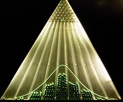
The bean machine, a device invented by Francis Galton, can be called the first generator of normal random variables. This machine consists of a vertical board with interleaved rows of pins. Small balls are dropped from the top and then bounce randomly left or right as they hit the pins. The balls are collected into bins at the bottom and settle down into a pattern resembling the Gaussian curve.

In computer simulations, especially in applications of the Monte-Carlo method, it is often desirable to generate values that are normally distributed. The algorithms listed below all generate the standard normal deviates, since a N(μ, σ²
) can be generated as X = μ + σZ, where Z is standard normal. All these algorithms rely on the availability of a random number generator U capable of producing uniform random variates.

The most straightforward method is based on the probability integral transform property: if U is distributed uniformly on (0,1), then Φ⁻¹(U) will have the standard normal distribution. The drawback of this method is that it relies on calculation of the probit function Φ⁻¹, which cannot be done analytically. Some approximate methods are described in Hart (1968) and in the erf article. Wichura gives a fast algorithm for computing this function to 16 decimal places,^[53] which is used by R to compute random variates of the normal distribution.

An easy to program approximate approach, that relies on the central limit theorem, is as follows: generate 12 uniform U(0,1) deviates, add them all up, and subtract 6 – the resulting random variable will have approximately standard normal distribution. In truth, the distribution will be Irwin–Hall, which is a 12-section eleventh-order polynomial approximation to the normal distribution. This random deviate will have a limited range of (−6, 6).^[54]

The Box–Muller method uses two independent random numbers U and V distributed uniformly on (0,1). Then the two random variables X and Y

X={sqrt {-2ln U}},cos(2pi V),qquad Y={sqrt {-2ln U}},sin(2pi V).

will both have the standard normal distribution, and will be independent. This formulation arises because for a bivariate normal random vector (X, Y) the squared norm X² + Y² will have the chi-squared distribution with two degrees of freedom, which is an easily generated exponential random variable corresponding to the quantity −2ln(U) in these equations; and the angle is distributed uniformly around the circle, chosen by the random variable V.

The Marsaglia polar method is a modification of the Box–Muller method which does not require computation of the sine and cosine functions. In this method, U and V are drawn from the uniform (−1,1) distribution, and then S = U² + V² is computed. If S is greater or equal to 1, then the method starts over, otherwise the two quantities

{displaystyle X=U{sqrt {frac {-2ln S}{S}}},qquad Y=V{sqrt {frac {-2ln S}{S}}}}

are returned. Again, X and Y are independent, standard normal random variables.

The Ratio method^[55] is a rejection method. The algorithm proceeds as follows:
- Generate two independent uniform deviates U and V;
- Compute X = √8/e (V − 0.5)/U;
- Optional: if X² ≤ 5 − 4e^1/4U then accept X and terminate algorithm;
- Optional: if X² ≥ 4e^−1.35/U + 1.4 then reject X and start over from step 1;
- If X² ≤ −4 lnU then accept X, otherwise start over the algorithm.

The two optional steps allow the evaluation of the logarithm in the last step to be avoided in most cases. These steps can be greatly improved^[56] so that the logarithm is rarely evaluated.

The ziggurat algorithm^[57] is faster than the Box–Muller transform and still exact. In about 97% of all cases it uses only two random numbers, one random integer and one random uniform, one multiplication and an if-test. Only in 3% of the cases, where the combination of those two falls outside the "core of the ziggurat" (a kind of rejection sampling using logarithms), do exponentials and more uniform random numbers have to be employed.

Integer arithmetic can be used to sample from the standard normal distribution.^[58] This method is exact in the sense that it satisfies the conditions of ideal approximation;^[59] i.e., it is equivalent to sampling a real number from the standard normal distribution and rounding this to the nearest representable floating point number.

There is also some investigation^[60] into the connection between the fast Hadamard transform and the normal distribution, since the transform employs just addition and subtraction and by the central limit theorem random numbers from almost any distribution will be transformed into the normal distribution. In this regard a series of Hadamard transforms can be combined with random permutations to turn arbitrary data sets into a normally distributed data.

Numerical approximations for the normal CDF

The standard normal CDF is widely used in scientific and statistical computing.

The values Φ(x) may be approximated very accurately by a variety of methods, such as numerical integration, Taylor series, asymptotic series and continued fractions. Different approximations are used depending on the desired level of accuracy.

Zelen & Severo (1964) give the approximation for Φ(x) for x > 0 with the absolute error |ε(x)| < 7.5·10⁻⁸ (algorithm 26.2.17):

${displaystyle Phi (x)=1-varphi (x)left(b_{1}t+b_{2}t^{2}+b_{3}t^{3}+b_{4}t^{4}+b_{5}t^{5}right)+varepsilon (x),qquad t={frac {1}{1+b_{0}x}},}$

where ϕ(x) is the standard normal PDF, and b₀ = 0.2316419, b₁ = 0.319381530, b₂ = −0.356563782, b₃ = 1.781477937, b₄ = −1.821255978, b₅ = 1.330274429.

Hart (1968) lists some dozens of approximations – by means of rational functions, with or without exponentials – for the .mw-parser-output .monospaced{font-family:monospace,monospace}
erfc() function. His algorithms vary in the degree of complexity and the resulting precision, with maximum absolute precision of 24 digits. An algorithm by West (2009) combines Hart's algorithm 5666 with a continued fraction approximation in the tail to provide a fast computation algorithm with a 16-digit precision.

Cody (1969) after recalling Hart68 solution is not suited for erf, gives a solution for both erf and erfc, with maximal relative error bound, via Rational Chebyshev Approximation.

Marsaglia (2004) suggested a simple algorithm^{[nb 1]} based on the Taylor series expansion

${displaystyle Phi (x)={frac {1}{2}}+varphi (x)left(x+{frac {x^{3}}{3}}+{frac {x^{5}}{3cdot 5}}+{frac {x^{7}}{3cdot 5cdot 7}}+{frac {x^{9}}{3cdot 5cdot 7cdot 9}}+cdots right)}$

for calculating Φ(x) with arbitrary precision. The drawback of this algorithm is comparatively slow calculation time (for example it takes over 300 iterations to calculate the function with 16 digits of precision when x = 10).

The GNU Scientific Library calculates values of the standard normal CDF using Hart's algorithms and approximations with Chebyshev polynomials.

Shore (1982) introduced simple approximations that may be incorporated in stochastic optimization models of engineering and operations research, like reliability engineering and inventory analysis. Denoting p=Φ(z), the simplest approximation for the quantile function is:

{displaystyle z=Phi ^{-1}(p)=5.5556left[1-left({frac {1-p}{p}}right)^{0.1186}right],qquad pgeq 1/2}

This approximation delivers for z a maximum absolute error of 0.026 (for 0.5 ≤ p ≤ 0.9999, corresponding to 0 ≤ z ≤ 3.719). For p < 1/2 replace p by 1 − p and change sign. Another approximation, somewhat less accurate, is the single-parameter approximation:

{displaystyle z=-0.4115left{{frac {1-p}{p}}+log left[{frac {1-p}{p}}right]-1right},qquad pgeq 1/2}

The latter had served to derive a simple approximation for the loss integral of the normal distribution, defined by

{displaystyle {begin{aligned}L(z)&=int _{z}^{infty }(u-z)varphi (u),du=int _{z}^{infty }[1-Phi (u)],du\[5pt]L(z)&approx {begin{cases}0.4115left({dfrac {p}{1-p}}right)-z,&p<1/2,\\0.4115left({dfrac {1-p}{p}}right),&pgeq 1/2.end{cases}}\[5pt]{text{or, equivalently,}}\L(z)&approx {begin{cases}0.4115left{1-log left[{frac {p}{1-p}}right]right},&p<1/2,\\0.4115{dfrac {1-p}{p}},&pgeq 1/2.end{cases}}end{aligned}}}

This approximation is particularly accurate for the right far-tail (maximum error of 10⁻³ for z≥1.4). Highly accurate approximations for the CDF, based on Response Modeling Methodology (RMM, Shore, 2011, 2012), are shown in Shore (2005).

Some more approximations can be found at: Error function#Approximation with elementary functions.

History

Development

Some authors^[61]^[62] attribute the credit for the discovery of the normal distribution to de Moivre, who in 1738^{[nb 2]} published in the second edition of his "The Doctrine of Chances" the study of the coefficients in the binomial expansion of (a + b)ⁿ. De Moivre proved that the middle term in this expansion has the approximate magnitude of $2/{sqrt {2pi n}}$ , and that "If m or ½n be a Quantity infinitely great, then the Logarithm of the Ratio, which a Term distant from the middle by the Interval ℓ, has to the middle Term, is $-{frac {2ell ell }{n}}$ ."^[63] Although this theorem can be interpreted as the first obscure expression for the normal probability law, Stigler points out that de Moivre himself did not interpret his results as anything more than the approximate rule for the binomial coefficients, and in particular de Moivre lacked the concept of the probability density function.^[64]

Carl Friedrich Gauss discovered the normal distribution in 1809 as a way to rationalize the method of least squares.

In 1809 Gauss published his monograph "Theoria motus corporum coelestium in sectionibus conicis solem ambientium" where among other things he introduces several important statistical concepts, such as the method of least squares, the method of maximum likelihood, and the normal distribution. Gauss used M, M′, M′′, … to denote the measurements of some unknown quantity V, and sought the "most probable" estimator of that quantity: the one that maximizes the probability φ(M − V) · φ(M′ − V) · φ(M′′ − V) · … of obtaining the observed experimental results. In his notation φΔ is the probability law of the measurement errors of magnitude Δ. Not knowing what the function φ is, Gauss requires that his method should reduce to the well-known answer: the arithmetic mean of the measured values.^{[nb 3]} Starting from these principles, Gauss demonstrates that the only law that rationalizes the choice of arithmetic mean as an estimator of the location parameter, is the normal law of errors:^[65]

{displaystyle varphi {mathit {Delta }}={frac {h}{surd pi }},e^{-mathrm {hh} Delta Delta },}

where h is "the measure of the precision of the observations". Using this normal law as a generic model for errors in the experiments, Gauss formulates what is now known as the non-linear weighted least squares (NWLS) method.^[66]

Marquis de Laplace proved the central limit theorem in 1810, consolidating the importance of the normal distribution in statistics.

Although Gauss was the first to suggest the normal distribution law, Laplace made significant contributions.^{[nb 4]} It was Laplace who first posed the problem of aggregating several observations in 1774,^[67] although his own solution led to the Laplacian distribution. It was Laplace who first calculated the value of the integral ∫ e^−t² dt = √ $π$ in 1782, providing the normalization constant for the normal distribution.^[68] Finally, it was Laplace who in 1810 proved and presented to the Academy the fundamental central limit theorem, which emphasized the theoretical importance of the normal distribution.^[69]

It is of interest to note that in 1809 an American mathematician Adrain published two derivations of the normal probability law, simultaneously and independently from Gauss.^[70] His works remained largely unnoticed by the scientific community, until in 1871 they were "rediscovered" by Abbe.^[71]

In the middle of the 19th century Maxwell demonstrated that the normal distribution is not just a convenient mathematical tool, but may also occur in natural phenomena:^[72] "The number of particles whose velocity, resolved in a certain direction, lies between x and x + dx is

{displaystyle operatorname {N} {frac {1}{alpha ;{sqrt {pi }}}};e^{-{frac {x^{2}}{alpha ^{2}}}},dx}

Naming

Since its introduction, the normal distribution has been known by many different names: the law of error, the law of facility of errors, Laplace's second law, Gaussian law, etc. Gauss himself apparently coined the term with reference to the "normal equations" involved in its applications, with normal having its technical meaning of orthogonal rather than "usual".^[73] However, by the end of the 19th century some authors^{[nb 5]} had started using the name normal distribution, where the word "normal" was used as an adjective – the term now being seen as a reflection of the fact that this distribution was seen as typical, common – and thus "normal". Peirce (one of those authors) once defined "normal" thus: "...the 'normal' is not the average (or any other kind of mean) of what actually occurs, but of what would, in the long run, occur under certain circumstances."^[74] Around the turn of the 20th century Pearson popularized the term normal as a designation for this distribution.^[75]

Many years ago I called the Laplace–Gaussian curve the normal curve, which name, while it avoids an international question of priority, has the disadvantage of leading people to believe that all other distributions of frequency are in one sense or another 'abnormal'.

— Pearson (1920)

Also, it was Pearson who first wrote the distribution in terms of the standard deviation σ as in modern notation. Soon after this, in year 1915, Fisher added the location parameter to the formula for normal distribution, expressing it in the way it is written nowadays:

{displaystyle df={frac {1}{sqrt {2sigma ^{2}pi }}}e^{-(x-m)^{2}/(2sigma ^{2})},dx}

The term "standard normal", which denotes the normal distribution with zero mean and unit variance came into general use around the 1950s, appearing in the popular textbooks by P.G. Hoel (1947) "Introduction to mathematical statistics" and A.M. Mood (1950) "Introduction to the theory of statistics".^[76]

When the name is used, the "Gaussian distribution" was named after Carl Friedrich Gauss, who introduced the distribution in 1809 as a way of rationalizing the method of least squares as outlined above. Among English speakers, both "normal distribution" and "Gaussian distribution" are in common use, with different terms preferred by different communities.

Notes

^ For example, this algorithm is given in the article Bc programming language.

^ De Moivre first published his findings in 1733, in a pamphlet "Approximatio ad Summam Terminorum Binomii (a + b)ⁿ in Seriem Expansi" that was designated for private circulation only. But it was not until the year 1738 that he made his results publicly available. The original pamphlet was reprinted several times, see for example Walker (1985).

^ "It has been customary certainly to regard as an axiom the hypothesis that if any quantity has been determined by several direct observations, made under the same circumstances and with equal care, the arithmetical mean of the observed values affords the most probable value, if not rigorously, yet very nearly at least, so that it is always most safe to adhere to it." — Gauss (1809, section 177)

^ "My custom of terming the curve the Gauss–Laplacian or normal curve saves us from proportioning the merit of discovery between the two great astronomer mathematicians." quote from Pearson (1905, p. 189)

^ Besides those specifically referenced here, such use is encountered in the works of Peirce, Galton (Galton (1889, chapter V)) and Lexis (Lexis (1878), Rohrbasser & Véron (2003)) c. 1875.^{[citation needed]}

References

Citations

^ Normal Distribution, Gale Encyclopedia of Psychology

^ Casella & Berger (2001, p. 102)

^ Lyon, A. (2014). Why are Normal Distributions Normal?, The British Journal for the Philosophy of Science.

^ For the proof see Gaussian integral

^ Stigler (1982)

^ Halperin, Hartley & Hoel (1965, item 7)

^ McPherson (1990, p. 110)

^ Bernardo & Smith (2000, p. 121)

^ Cover, Thomas M.; Thomas, Joy A. (2006). Elements of Information Theory. John Wiley and Sons. p. 254..mw-parser-output cite.citation{font-style:inherit}.mw-parser-output q{quotes:"""""""'""'"}.mw-parser-output code.cs1-code{color:inherit;background:inherit;border:inherit;padding:inherit}.mw-parser-output .cs1-lock-free a{background:url("//upload.wikimedia.org/wikipedia/commons/thumb/6/65/Lock-green.svg/9px-Lock-green.svg.png")no-repeat;background-position:right .1em center}.mw-parser-output .cs1-lock-limited a,.mw-parser-output .cs1-lock-registration a{background:url("//upload.wikimedia.org/wikipedia/commons/thumb/d/d6/Lock-gray-alt-2.svg/9px-Lock-gray-alt-2.svg.png")no-repeat;background-position:right .1em center}.mw-parser-output .cs1-lock-subscription a{background:url("//upload.wikimedia.org/wikipedia/commons/thumb/a/aa/Lock-red-alt-2.svg/9px-Lock-red-alt-2.svg.png")no-repeat;background-position:right .1em center}.mw-parser-output .cs1-subscription,.mw-parser-output .cs1-registration{color:#555}.mw-parser-output .cs1-subscription span,.mw-parser-output .cs1-registration span{border-bottom:1px dotted;cursor:help}.mw-parser-output .cs1-hidden-error{display:none;font-size:100%}.mw-parser-output .cs1-visible-error{font-size:100%}.mw-parser-output .cs1-subscription,.mw-parser-output .cs1-registration,.mw-parser-output .cs1-format{font-size:95%}.mw-parser-output .cs1-kern-left,.mw-parser-output .cs1-kern-wl-left{padding-left:0.2em}.mw-parser-output .cs1-kern-right,.mw-parser-output .cs1-kern-wl-right{padding-right:0.2em}

^ Park, Sung Y.; Bera, Anil K. (2009). "Maximum Entropy Autoregressive Conditional Heteroskedasticity Model" (PDF). Journal of Econometrics. Elsevier. 150 (2): 219–230. doi:10.1016/j.jeconom.2008.12.014. Retrieved 2011-06-02.

^ Geary RC(1936) The distribution of the "Student's" ratio for the non-normal samples". Supplement to the Journal of the Royal Statistical Society 3 (2): 178–184

^ Lukas E (1942) A characterization of the normal distribution. Annals of Mathematical Statistics 13: 91–93

^ ^a^b^c Patel & Read (1996, [2.1.4])

^ Fan (1991, p. 1258)

^ Patel & Read (1996, [2.1.8])

^ Papoulis, Athanasios. Probability, Random Variables and Stochastic Processes (4th Edition). p. 148.

^ Bryc (1995, p. 23)

^ Bryc (1995, p. 24)

^ Scott, Clayton; Nowak, Robert (August 7, 2003). "The Q-function". Connexions.

^ Barak, Ohad (April 6, 2006). "Q Function and Error Function" (PDF). Tel Aviv University. Archived from the original (PDF) on March 25, 2009.

^ Weisstein, Eric W. "Normal Distribution Function". MathWorld.

^ Abramowitz, Milton; Stegun, Irene Ann, eds. (1983) [June 1964]. "Chapter 26, eqn 26.2.12". Handbook of Mathematical Functions with Formulas, Graphs, and Mathematical Tables. Applied Mathematics Series. 55 (Ninth reprint with additional corrections of tenth original printing with corrections (December 1972); first ed.). Washington D.C.; New York: United States Department of Commerce, National Bureau of Standards; Dover Publications. p. 932. ISBN 978-0-486-61272-0. LCCN 64-60036. MR 0167642. LCCN 65-12253.

^ "Wolfram|Alpha: Computational Knowledge Engine". Wolframalpha.com. Retrieved 2017-03-03.

^ "Wolfram|Alpha: Computational Knowledge Engine". Wolframalpha.com.

^ "Wolfram|Alpha: Computational Knowledge Engine". Wolframalpha.com. Retrieved 2017-03-03.

^ "Normal Approximation to Poisson Distribution". Stat.ucla.edu. Retrieved 2017-03-03.

^ Cover & Thomas (2006, p. 254)

^ Williams, David (2001). Weighing the odds : a course in probability and statistics (Reprinted. ed.). Cambridge [u.a.]: Cambridge Univ. Press. pp. 197–199. ISBN 0-521-00618-X.

^ Smith, José M. Bernardo; Adrian F. M. (2000). Bayesian theory (Reprint ed.). Chichester [u.a.]: Wiley. pp. 209, 366. ISBN 0-471-49464-X.

^ O'Hagan, A. (1994) Kendall's Advanced Theory of statistics, Vol 2B, Bayesian Inference, Edward Arnold.
ISBN 0-340-52922-9 (Section 5.40)

^ Bryc (1995, p. 27)

^ Patel & Read (1996, [2.3.6])

^ Galambos & Simonelli (2004, Theorem 3.5)

^ ^a^b Bryc (1995, p. 35)

^ ^a^b Lukacs & King (1954)

^ Quine, M.P. (1993). "On three characterisations of the normal distribution". Probability and Mathematical Statistics. 14 (2): 257–263.

^ UIUC, Lecture 21. The Multivariate Normal Distribution, 21.6:"Individually Gaussian Versus Jointly Gaussian".

^ Edward L. Melnick and Aaron Tenenbein, "Misspecifications of the Normal Distribution", The American Statistician, volume 36, number 4 November 1982, pages 372–373

^ "Kullback Leibler (KL) Distance of Two Normal (Gaussian) Probability Distributions". Allisons.org. 2007-12-05. Retrieved 2017-03-03.

^ Jordan, Michael I. (February 8, 2010). "Stat260: Bayesian Modeling and Inference: The Conjugate Prior for the Normal Distribution" (PDF).

^ Amari & Nagaoka (2000)

^ Weisstein, Eric W. "Normal Product Distribution". MathWorld. wolfram.com.

^ Lukacs, Eugene (1942). "A Characterization of the Normal Distribution". The Annals of Mathematical Statistics. Institute of Mathematical Statistics. 13 (1): 91–3. doi:10.1214/aoms/1177731647. ISSN 0003-4851. JSTOR 2236166. (Registration required (help)).

^ Basu, D.; Laha, R. G. (1954). "On Some Characterizations of the Normal Distribution". Sankhyā. Indian Statistical Institute. 13 (4): 359–62. ISSN 0036-4452. JSTOR 25048183. (Registration required (help)).

^ Lehmann, E. L. (1997). Testing Statistical Hypotheses (2nd ed.). Springer. p. 199. ISBN 0-387-94919-4.

^ John, S (1982). "The three parameter two-piece normal family of distributions and its fitting". Communications in statistics - Theory and Methods. 11 (8): 879–885. doi:10.1080/03610928208828279.

^ ^a^b Krishnamoorthy (2006, p. 127)

^ Krishnamoorthy (2006, p. 130)

^ Krishnamoorthy (2006, p. 133)

^ Huxley (1932)

^ Jaynes, Edwin T. (2003). Probability Theory: The Logic of Science. Cambridge University Press. pp. 592–593.

^ Oosterbaan, Roland J. (1994). "Chapter 6: Frequency and Regression Analysis of Hydrologic Data". In Ritzema, Henk P. Drainage Principles and Applications, Publication 16 (PDF) (second revised ed.). Wageningen, The Netherlands: International Institute for Land Reclamation and Improvement (ILRI). pp. 175–224. ISBN 90-70754-33-9.

^ Wichura, Michael J. (1988). "Algorithm AS241: The Percentage Points of the Normal Distribution". Applied Statistics. Blackwell Publishing. 37 (3): 477–84. doi:10.2307/2347330. JSTOR 2347330. (Registration required (help)).

^ Johnson, Kotz & Balakrishnan (1995, Equation (26.48))

^ Kinderman & Monahan (1977)

^ Leva (1992)

^ Marsaglia & Tsang (2000)

^ Karney (2016)

^ Monahan (1985, section 2)

^ Wallace (1996)

^ Johnson, Kotz & Balakrishnan (1994, p. 85)

^ Le Cam & Lo Yang (2000, p. 74)

^ De Moivre, Abraham (1733), Corollary I – see Walker (1985, p. 77)

^ Stigler (1986, p. 76)

^ Gauss (1809, section 177)

^ Gauss (1809, section 179)

^ Laplace (1774, Problem III)

^ Pearson (1905, p. 189)

^ Stigler (1986, p. 144)

^ Stigler (1978, p. 243)

^ Stigler (1978, p. 244)

^ Maxwell (1860, p. 23)

^ Jaynes, Edwin J.; Probability Theory: The Logic of Science, Ch 7

^ Peirce, Charles S. (c. 1909 MS), Collected Papers v. 6, paragraph 327

^ Kruskal & Stigler (1997)

^ "Earliest uses… (entry STANDARD NORMAL CURVE)".

Sources

.mw-parser-output .refbegin{font-size:90%;margin-bottom:0.5em}.mw-parser-output .refbegin-hanging-indents>ul{list-style-type:none;margin-left:0}.mw-parser-output .refbegin-hanging-indents>ul>li,.mw-parser-output .refbegin-hanging-indents>dl>dd{margin-left:0;padding-left:3.2em;text-indent:-3.2em;list-style:none}.mw-parser-output .refbegin-100{font-size:100%}

Aldrich, John; Miller, Jeff. "Earliest Uses of Symbols in Probability and Statistics".

Aldrich, John; Miller, Jeff. "Earliest Known Uses of Some of the Words of Mathematics". In particular, the entries for "bell-shaped and bell curve", "normal (distribution)", "Gaussian", and "Error, law of error, theory of errors, etc.".

Amari, Shun-ichi; Nagaoka, Hiroshi (2000). Methods of Information Geometry. Oxford University Press. ISBN 0-8218-0531-2.

Bernardo, José M.; Smith, Adrian F. M. (2000). Bayesian Theory. Wiley. ISBN 0-471-49464-X.

Bryc, Wlodzimierz (1995). The Normal Distribution: Characterizations with Applications. Springer-Verlag. ISBN 0-387-97990-5.

Casella, George; Berger, Roger L. (2001). Statistical Inference (2nd ed.). Duxbury. ISBN 0-534-24312-6.

Cody, William J. (1969). "Rational Chebyshev Approximations for the Error Function". Mathematics of Computation. 23 (107): 631–638. doi:10.1090/S0025-5718-1969-0247736-4.

Cover, Thomas M.; Thomas, Joy A. (2006). Elements of Information Theory. John Wiley and Sons.

de Moivre, Abraham (1738). The Doctrine of Chances. ISBN 0-8218-2103-2.

Fan, Jianqing (1991). "On the optimal rates of convergence for nonparametric deconvolution problems". The Annals of Statistics. 19 (3): 1257–1272. doi:10.1214/aos/1176348248. JSTOR 2241949.

Galton, Francis (1889). Natural Inheritance (PDF). London, UK: Richard Clay and Sons.

Galambos, Janos; Simonelli, Italo (2004). Products of Random Variables: Applications to Problems of Physics and to Arithmetical Functions. Marcel Dekker, Inc. ISBN 0-8247-5402-6.

Gauss, Carolo Friderico (1809). Theoria motvs corporvm coelestivm in sectionibvs conicis Solem ambientivm [Theory of the Motion of the Heavenly Bodies Moving about the Sun in Conic Sections] (in Latin). English translation.

Gould, Stephen Jay (1981). The Mismeasure of Man (first ed.). W. W. Norton. ISBN 0-393-01489-4.

Halperin, Max; Hartley, Herman O.; Hoel, Paul G. (1965). "Recommended Standards for Statistical Symbols and Notation. COPSS Committee on Symbols and Notation". The American Statistician. 19 (3): 12–14. doi:10.2307/2681417. JSTOR 2681417.

Hart, John F.; et al. (1968). Computer Approximations. New York, NY: John Wiley & Sons, Inc. ISBN 0-88275-642-7.

Hazewinkel, Michiel, ed. (2001) [1994], "Normal Distribution", Encyclopedia of Mathematics, Springer Science+Business Media B.V. / Kluwer Academic Publishers, ISBN 978-1-55608-010-4

Herrnstein, Richard J.; Murray, Charles (1994). The Bell Curve: Intelligence and Class Structure in American Life. Free Press. ISBN 0-02-914673-9.

Huxley, Julian S. (1932). Problems of Relative Growth. London. ISBN 0-486-61114-0. OCLC 476909537.

Johnson, Norman L.; Kotz, Samuel; Balakrishnan, Narayanaswamy (1994). Continuous Univariate Distributions, Volume 1. Wiley. ISBN 0-471-58495-9.

Johnson, Norman L.; Kotz, Samuel; Balakrishnan, Narayanaswamy (1995). Continuous Univariate Distributions, Volume 2. Wiley. ISBN 0-471-58494-0.

Karney, C. F. F. (2016). "Sampling exactly from the normal distribution". ACM Transactions on Mathematical Software. 42 (1): 3:1–14. arXiv:1303.6257. doi:10.1145/2710016.

Kinderman, Albert J.; Monahan, John F. (1977). "Computer Generation of Random Variables Using the Ratio of Uniform Deviates". ACM Transactions on Mathematical Software. 3 (3): 257–260. doi:10.1145/355744.355750.

Krishnamoorthy, Kalimuthu (2006). Handbook of Statistical Distributions with Applications. Chapman & Hall/CRC. ISBN 1-58488-635-8.

Kruskal, William H.; Stigler, Stephen M. (1997). Spencer, Bruce D., ed. Normative Terminology: 'Normal' in Statistics and Elsewhere. Statistics and Public Policy. Oxford University Press. ISBN 0-19-852341-6.

Laplace, Pierre-Simon de (1774). "Mémoire sur la probabilité des causes par les événements". Mémoires de l'Académie royale des Sciences de Paris (Savants étrangers), tome 6: 621–656. Translated by Stephen M. Stigler in Statistical Science 1 (3), 1986: JSTOR 2245476.

Laplace, Pierre-Simon (1812). Théorie analytique des probabilités [Analytical theory of probabilities].

Le Cam, Lucien; Lo Yang, Grace (2000). Asymptotics in Statistics: Some Basic Concepts (second ed.). Springer. ISBN 0-387-95036-2.

Leva, Joseph L. (1992). "A fast normal random number generator" (PDF). ACM Transactions on Mathematical Software. 18 (4): 449–453. doi:10.1145/138351.138364. Archived from the original (PDF) on 16 July 2010.

Lexis, Wilhelm (1878). "Sur la durée normale de la vie humaine et sur la théorie de la stabilité des rapports statistiques". Annales de démographie internationale. Paris. II: 447–462.

Lukacs, Eugene; King, Edgar P. (1954). "A Property of Normal Distribution". The Annals of Mathematical Statistics. 25 (2): 389–394. doi:10.1214/aoms/1177728796. JSTOR 2236741.

McPherson, Glen (1990). Statistics in Scientific Investigation: Its Basis, Application and Interpretation. Springer-Verlag. ISBN 0-387-97137-8.

Marsaglia, George; Tsang, Wai Wan (2000). "The Ziggurat Method for Generating Random Variables". Journal of Statistical Software. 5 (8). doi:10.18637/jss.v005.i08.

Marsaglia, George (2004). "Evaluating the Normal Distribution". Journal of Statistical Software. 11 (4). doi:10.18637/jss.v011.i04.

Maxwell, James Clerk (1860). "V. Illustrations of the dynamical theory of gases. — Part I: On the motions and collisions of perfectly elastic spheres". Philosophical Magazine. Series 4. 19 (124): 19–32. doi:10.1080/14786446008642818.

Monahan, J. F. (1985). "Accuracy in random number generation". Mathematics of Computation. 45 (172): 559–568. doi:10.1090/S0025-5718-1985-0804945-X.

Patel, Jagdish K.; Read, Campbell B. (1996). Handbook of the Normal Distribution (2nd ed.). CRC Press. ISBN 0-8247-9342-0.

Pearson, Karl (1901). "On Lines and Planes of Closest Fit to Systems of Points in Space" (PDF). Philosophical Magazine. 6. 2: 559–572. doi:10.1080/14786440109462720.

Pearson, Karl (1905). "'Das Fehlergesetz und seine Verallgemeinerungen durch Fechner und Pearson'. A rejoinder". Biometrika. 4 (1): 169–212. doi:10.2307/2331536. JSTOR 2331536.

Pearson, Karl (1920). "Notes on the History of Correlation". Biometrika. 13 (1): 25–45. doi:10.1093/biomet/13.1.25. JSTOR 2331722.

Rohrbasser, Jean-Marc; Véron, Jacques (2003). "Wilhelm Lexis: The Normal Length of Life as an Expression of the "Nature of Things"". Population. 58 (3): 303–322. doi:10.3917/pope.303.0303.

Shore, H (1982). "Simple Approximations for the Inverse Cumulative Function, the Density Function and the Loss Integral of the Normal Distribution". Journal of the Royal Statistical Society. Series C (Applied Statistics). 31 (2): 108–114. doi:10.2307/2347972.

Shore, H (2005). "Accurate RMM-Based Approximations for the CDF of the Normal Distribution". Communications in Statistics – Theory and Methods. 34: 507–513. doi:10.1081/sta-200052102.

Shore, H (2011). "Response Modeling Methodology". WIREs Comput Stat. 3: 357–372. doi:10.1002/wics.151.

Shore, H (2012). "Estimating Response Modeling Methodology Models". WIREs Comput Stat. 4: 323–333. doi:10.1002/wics.1199.

Stigler, Stephen M. (1978). "Mathematical Statistics in the Early States". The Annals of Statistics. 6 (2): 239–265. doi:10.1214/aos/1176344123. JSTOR 2958876.

Stigler, Stephen M. (1982). "A Modest Proposal: A New Standard for the Normal". The American Statistician. 36 (2): 137–138. doi:10.2307/2684031. JSTOR 2684031.

Stigler, Stephen M. (1986). The History of Statistics: The Measurement of Uncertainty before 1900. Harvard University Press. ISBN 0-674-40340-1.

Stigler, Stephen M. (1999). Statistics on the Table. Harvard University Press. ISBN 0-674-83601-4.

Walker, Helen M. (1985). "De Moivre on the Law of Normal Probability" (PDF). In Smith, David Eugene. A Source Book in Mathematics. Dover. ISBN 0-486-64690-4.

Wallace, C. S. (1996). "Fast pseudo-random generators for normal and exponential variates". ACM Transactions on Mathematical Software. 22 (1): 119–127. doi:10.1145/225545.225554.

Weisstein, Eric W. "Normal Distribution". MathWorld.

West, Graeme (2009). "Better Approximations to Cumulative Normal Functions" (PDF). Wilmott Magazine: 70–76.

Zelen, Marvin; Severo, Norman C. (1964). Probability Functions (chapter 26). Handbook of mathematical functions with formulas, graphs, and mathematical tables, by Abramowitz, M.; and Stegun, I. A.: National Bureau of Standards. New York, NY: Dover. ISBN 0-486-61272-4.

External links

Hazewinkel, Michiel, ed. (2001) [1994], "Normal distribution", Encyclopedia of Mathematics, Springer Science+Business Media B.V. / Kluwer Academic Publishers, ISBN 978-1-55608-010-4

Normal Distribution Video Tutorial Part 1-2 on YouTube

Normal distribution calculator

An 8-foot-tall (2.4 m) Probability Machine (named Sir Francis) comparing stock market returns to the randomness of the beans dropping through the quincunx pattern. on YouTube Link originating from Index Fund Advisors

[61] For example, this algorithm is given in the article Bc programming language.

[64] De Moivre first published his findings in 1733, in a pamphlet "Approximatio ad Summam Terminorum Binomii (a + b)ⁿ in Seriem Expansi" that was designated for private circulation only. But it was not until the year 1738 that he made his results publicly available. The original pamphlet was reprinted several times, see for example Walker (1985).

[67] "It has been customary certainly to regard as an axiom the hypothesis that if any quantity has been determined by several direct observations, made under the same circumstances and with equal care, the arithmetical mean of the observed values affords the most probable value, if not rigorously, yet very nearly at least, so that it is always most safe to adhere to it." — Gauss (1809, section 177)

[70] "My custom of terming the curve the Gauss–Laplacian or normal curve saves us from proportioning the merit of discovery between the two great astronomer mathematicians." quote from Pearson (1905, p. 189)

[78] Besides those specifically referenced here, such use is encountered in the works of Peirce, Galton (Galton (1889, chapter V)) and Lexis (Lexis (1878), Rohrbasser & Véron (2003)) c. 1875.^{[citation needed]}

[1] Normal Distribution, Gale Encyclopedia of Psychology

[2] Casella & Berger (2001, p. 102)

[3] Lyon, A. (2014). Why are Normal Distributions Normal?, The British Journal for the Philosophy of Science.

[4] For the proof see Gaussian integral

[5] Stigler (1982)

[6] Halperin, Hartley & Hoel (1965, item 7)

[7] McPherson (1990, p. 110)

[8] Bernardo & Smith (2000, p. 121)

[9] Cover, Thomas M.; Thomas, Joy A. (2006). Elements of Information Theory. John Wiley and Sons. p. 254..mw-parser-output cite.citation{font-style:inherit}.mw-parser-output q{quotes:"""""""'""'"}.mw-parser-output code.cs1-code{color:inherit;background:inherit;border:inherit;padding:inherit}.mw-parser-output .cs1-lock-free a{background:url("//upload.wikimedia.org/wikipedia/commons/thumb/6/65/Lock-green.svg/9px-Lock-green.svg.png")no-repeat;background-position:right .1em center}.mw-parser-output .cs1-lock-limited a,.mw-parser-output .cs1-lock-registration a{background:url("//upload.wikimedia.org/wikipedia/commons/thumb/d/d6/Lock-gray-alt-2.svg/9px-Lock-gray-alt-2.svg.png")no-repeat;background-position:right .1em center}.mw-parser-output .cs1-lock-subscription a{background:url("//upload.wikimedia.org/wikipedia/commons/thumb/a/aa/Lock-red-alt-2.svg/9px-Lock-red-alt-2.svg.png")no-repeat;background-position:right .1em center}.mw-parser-output .cs1-subscription,.mw-parser-output .cs1-registration{color:#555}.mw-parser-output .cs1-subscription span,.mw-parser-output .cs1-registration span{border-bottom:1px dotted;cursor:help}.mw-parser-output .cs1-hidden-error{display:none;font-size:100%}.mw-parser-output .cs1-visible-error{font-size:100%}.mw-parser-output .cs1-subscription,.mw-parser-output .cs1-registration,.mw-parser-output .cs1-format{font-size:95%}.mw-parser-output .cs1-kern-left,.mw-parser-output .cs1-kern-wl-left{padding-left:0.2em}.mw-parser-output .cs1-kern-right,.mw-parser-output .cs1-kern-wl-right{padding-right:0.2em}

[10] Park, Sung Y.; Bera, Anil K. (2009). "Maximum Entropy Autoregressive Conditional Heteroskedasticity Model" (PDF). Journal of Econometrics. Elsevier. 150 (2): 219–230. doi:10.1016/j.jeconom.2008.12.014. Retrieved 2011-06-02.

[Geary1936-11] Geary RC(1936) The distribution of the "Student's" ratio for the non-normal samples". Supplement to the Journal of the Royal Statistical Society 3 (2): 178–184

[Lukas1942-12] Lukas E (1942) A characterization of the normal distribution. Annals of Mathematical Statistics 13: 91–93

[PR2.1.4-13] Patel & Read (1996, [2.1.4])

[14] Fan (1991, p. 1258)

[15] Patel & Read (1996, [2.1.8])

[16] Papoulis, Athanasios. Probability, Random Variables and Stochastic Processes (4th Edition). p. 148.

[17] Bryc (1995, p. 23)

[18] Bryc (1995, p. 24)

[19] Scott, Clayton; Nowak, Robert (August 7, 2003). "The Q-function". Connexions.

[20] Barak, Ohad (April 6, 2006). "Q Function and Error Function" (PDF). Tel Aviv University. Archived from the original (PDF) on March 25, 2009.

[21] Weisstein, Eric W. "Normal Distribution Function". MathWorld.

[22] Abramowitz, Milton; Stegun, Irene Ann, eds. (1983) [June 1964]. "Chapter 26, eqn 26.2.12". Handbook of Mathematical Functions with Formulas, Graphs, and Mathematical Tables. Applied Mathematics Series. 55 (Ninth reprint with additional corrections of tenth original printing with corrections (December 1972); first ed.). Washington D.C.; New York: United States Department of Commerce, National Bureau of Standards; Dover Publications. p. 932. ISBN 978-0-486-61272-0. LCCN 64-60036. MR 0167642. LCCN 65-12253.

[23] "Wolfram|Alpha: Computational Knowledge Engine". Wolframalpha.com. Retrieved 2017-03-03.

[24] "Wolfram|Alpha: Computational Knowledge Engine". Wolframalpha.com.

[25] "Wolfram|Alpha: Computational Knowledge Engine". Wolframalpha.com. Retrieved 2017-03-03.

[26] "Normal Approximation to Poisson Distribution". Stat.ucla.edu. Retrieved 2017-03-03.

[27] Cover & Thomas (2006, p. 254)

[28] Williams, David (2001). Weighing the odds : a course in probability and statistics (Reprinted. ed.). Cambridge [u.a.]: Cambridge Univ. Press. pp. 197–199. ISBN 0-521-00618-X.

[29] Smith, José M. Bernardo; Adrian F. M. (2000). Bayesian theory (Reprint ed.). Chichester [u.a.]: Wiley. pp. 209, 366. ISBN 0-471-49464-X.

[30] O'Hagan, A. (1994) Kendall's Advanced Theory of statistics, Vol 2B, Bayesian Inference, Edward Arnold.
ISBN 0-340-52922-9 (Section 5.40)

[31] Bryc (1995, p. 27)

[32] Patel & Read (1996, [2.3.6])

[33] Galambos & Simonelli (2004, Theorem 3.5)

[Bryc_1995_35-34] Bryc (1995, p. 35)

[LK-35] Lukacs & King (1954)

[36] Quine, M.P. (1993). "On three characterisations of the normal distribution". Probability and Mathematical Statistics. 14 (2): 257–263.

[37] UIUC, Lecture 21. The Multivariate Normal Distribution, 21.6:"Individually Gaussian Versus Jointly Gaussian".

[38] Edward L. Melnick and Aaron Tenenbein, "Misspecifications of the Normal Distribution", The American Statistician, volume 36, number 4 November 1982, pages 372–373

[39] "Kullback Leibler (KL) Distance of Two Normal (Gaussian) Probability Distributions". Allisons.org. 2007-12-05. Retrieved 2017-03-03.

[40] Jordan, Michael I. (February 8, 2010). "Stat260: Bayesian Modeling and Inference: The Conjugate Prior for the Normal Distribution" (PDF).

[41] Amari & Nagaoka (2000)

[42] Weisstein, Eric W. "Normal Product Distribution". MathWorld. wolfram.com.

[43] Lukacs, Eugene (1942). "A Characterization of the Normal Distribution". The Annals of Mathematical Statistics. Institute of Mathematical Statistics. 13 (1): 91–3. doi:10.1214/aoms/1177731647. ISSN 0003-4851. JSTOR 2236166. (Registration required (help)).

[44] Basu, D.; Laha, R. G. (1954). "On Some Characterizations of the Normal Distribution". Sankhyā. Indian Statistical Institute. 13 (4): 359–62. ISSN 0036-4452. JSTOR 25048183. (Registration required (help)).

[45] Lehmann, E. L. (1997). Testing Statistical Hypotheses (2nd ed.). Springer. p. 199. ISBN 0-387-94919-4.

[John1982-46] John, S (1982). "The three parameter two-piece normal family of distributions and its fitting". Communications in statistics - Theory and Methods. 11 (8): 879–885. doi:10.1080/03610928208828279.

[Kri127-47] Krishnamoorthy (2006, p. 127)

[48] Krishnamoorthy (2006, p. 130)

[49] Krishnamoorthy (2006, p. 133)

[50] Huxley (1932)

[51] Jaynes, Edwin T. (2003). Probability Theory: The Logic of Science. Cambridge University Press. pp. 592–593.

[52] Oosterbaan, Roland J. (1994). "Chapter 6: Frequency and Regression Analysis of Hydrologic Data". In Ritzema, Henk P. Drainage Principles and Applications, Publication 16 (PDF) (second revised ed.). Wageningen, The Netherlands: International Institute for Land Reclamation and Improvement (ILRI). pp. 175–224. ISBN 90-70754-33-9.

[53] Wichura, Michael J. (1988). "Algorithm AS241: The Percentage Points of the Normal Distribution". Applied Statistics. Blackwell Publishing. 37 (3): 477–84. doi:10.2307/2347330. JSTOR 2347330. (Registration required (help)).

[54] Johnson, Kotz & Balakrishnan (1995, Equation (26.48))

[55] Kinderman & Monahan (1977)

[56] Leva (1992)

[57] Marsaglia & Tsang (2000)

[58] Karney (2016)

[59] Monahan (1985, section 2)

[60] Wallace (1996)

[62] Johnson, Kotz & Balakrishnan (1994, p. 85)

[63] Le Cam & Lo Yang (2000, p. 74)

[65] De Moivre, Abraham (1733), Corollary I – see Walker (1985, p. 77)

[66] Stigler (1986, p. 76)

[68] Gauss (1809, section 177)

[69] Gauss (1809, section 179)

[71] Laplace (1774, Problem III)

[72] Pearson (1905, p. 189)

[73] Stigler (1986, p. 144)

[74] Stigler (1978, p. 243)

[75] Stigler (1978, p. 244)

[76] Maxwell (1860, p. 23)

[77] Jaynes, Edwin J.; Probability Theory: The Logic of Science, Ch 7

[79] Peirce, Charles S. (c. 1909 MS), Collected Papers v. 6, paragraph 327

[80] Kruskal & Stigler (1997)

[81] "Earliest uses… (entry STANDARD NORMAL CURVE)".

v t e Probability distributions
List
Discrete univariate with finite support	Benford Bernoulli beta-binomial binomial categorical hypergeometric Poisson binomial Rademacher soliton discrete uniform Zipf Zipf–Mandelbrot
Discrete univariate with infinite support	beta negative binomial Borel Conway–Maxwell–Poisson discrete phase-type Delaporte extended negative binomial Gauss–Kuzmin geometric logarithmic negative binomial parabolic fractal Poisson Skellam Yule–Simon zeta
Continuous univariate supported on a bounded interval	arcsine ARGUS Balding–Nichols Bates beta beta rectangular Irwin–Hall Kumaraswamy logit-normal noncentral beta raised cosine reciprocal triangular U-quadratic uniform Wigner semicircle
Continuous univariate supported on a semi-infinite interval	Benini Benktander 1st kind Benktander 2nd kind beta prime Burr chi-squared chi Dagum Davis exponential-logarithmic Erlang exponential F folded normal Flory–Schulz Fréchet gamma gamma/Gompertz generalized inverse Gaussian Gompertz half-logistic half-normal Hotelling's T-squared hyper-Erlang hyperexponential hypoexponential inverse chi-squared scaled inverse chi-squared inverse Gaussian inverse gamma Kolmogorov Lévy log-Cauchy log-Laplace log-logistic log-normal Lomax matrix-exponential Maxwell–Boltzmann Maxwell–Jüttner Mittag-Leffler Nakagami noncentral chi-squared Pareto phase-type poly-Weibull Rayleigh relativistic Breit–Wigner Rice shifted Gompertz truncated normal type-2 Gumbel Weibull Discrete Weibull Wilks's lambda
Continuous univariate supported on the whole real line	Cauchy exponential power Fisher's z Gaussian q generalized normal generalized hyperbolic geometric stable Gumbel Holtsmark hyperbolic secant Johnson's S_U Landau Laplace asymmetric Laplace logistic noncentral t normal (Gaussian) normal-inverse Gaussian skew normal slash stable Student's t type-1 Gumbel Tracy–Widom variance-gamma Voigt
Continuous univariate with support whose type varies	generalized extreme value generalized Pareto Marchenko–Pastur q-exponential q-Gaussian q-Weibull shifted log-logistic Tukey lambda
Mixed continuous-discrete univariate	rectified Gaussian
Multivariate (joint)	.mw-parser-output .nobold{font-weight:normal} Discrete Ewens multinomial Dirichlet-multinomial negative multinomial Continuous Dirichlet generalized Dirichlet multivariate Laplace multivariate normal multivariate stable multivariate t normal-inverse-gamma normal-gamma Matrix-valued inverse matrix gamma inverse-Wishart matrix normal matrix t matrix gamma normal-inverse-Wishart normal-Wishart Wishart
Directional	Univariate (circular) directional Circular uniform univariate von Mises wrapped normal wrapped Cauchy wrapped exponential wrapped asymmetric Laplace wrapped Lévy Bivariate (spherical) Kent Bivariate (toroidal) bivariate von Mises Multivariate von Mises–Fisher Bingham
Degenerate and singular	Degenerate Dirac delta function Singular Cantor
Families	Circular compound Poisson elliptical exponential natural exponential location–scale maximum entropy mixture Pearson Tweedie wrapped

Probability density function The red curve is the standard normal distribution
Cumulative distribution function
Notation	${mathcal {N}}(mu ,sigma ^{2})$
Parameters	${displaystyle mu in mathbb {R} }$ = mean (location) $sigma ^{2}>0$ = variance (squared scale)
Support	${displaystyle xin mathbb {R} }$
PDF	${displaystyle {frac {1}{sqrt {2pi sigma ^{2}}}}e^{-{frac {(x-mu )^{2}}{2sigma ^{2}}}}}$
CDF	${displaystyle {frac {1}{2}}left[1+operatorname {erf} left({frac {x-mu }{sigma {sqrt {2}}}}right)right]}$
Quantile	${displaystyle mu +sigma {sqrt {2}}operatorname {erf} ^{-1}(2F-1)}$
Mean	$mu$
Median	$mu$
Mode	$mu$
Variance	$sigma ^{2}$
Skewness	${displaystyle 0}$
Ex. kurtosis	${displaystyle 0}$
Entropy	${displaystyle {frac {1}{2}}log(2pi esigma ^{2})}$
MGF	${displaystyle exp(mu t+sigma ^{2}t^{2}/2)}$
CF	${displaystyle exp(imu t-sigma ^{2}t^{2}/2)}$
Fisher information	${displaystyle {mathcal {I}}(mu ,sigma )={begin{pmatrix}1/sigma ^{2}&0\0&2/sigma ^{2}end{pmatrix}}}$ ${displaystyle {mathcal {I}}(mu ,sigma ^{2})={begin{pmatrix}1/sigma ^{2}&0\0&1/(2sigma ^{4})end{pmatrix}}}$

Normal distribution

Contents

Definition

Standard normal distribution

General normal distribution

Notation

Alternative parameterizations

Properties

Symmetries and derivatives

Moments

Fourier transform and characteristic function

Moment and cumulant generating functions

Cumulative distribution function

Standard deviation and coverage

Quantile function

Zero-variance limit

Central limit theorem

Maximum entropy

Operations on normal deviates

Infinite divisibility and Cramér's theorem

Bernstein's theorem

Other properties

Related distributions

Operations on a single random variable

Combination of two independent random variables

Combination of two or more independent random variables

Operations on the density function

Extensions

Normality tests

Estimation of parameters

Sample mean

Sample variance

Confidence intervals

Bayesian analysis of the normal distribution

Sum of two quadratics

Scalar form

Vector form

Sum of differences from the mean

With known variance

With known mean

With unknown mean and unknown variance

Occurrence and applications

Exact normality

Approximate normality

Assumed normality

Produced normality

Generating values from normal distribution

Numerical approximations for the normal CDF

History

Development

Naming

See also

Notes

References

Citations

Sources

External links

Popular posts from this blog

鏡平學校

Why https connections are so slow when debugging (stepping over) in Java?