Agfdhyk

Uniform

Probability density function 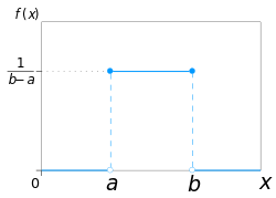Using maximum convention
Cumulative distribution function
Notation	U(a,b){displaystyle {mathcal {U}}(a,b)} or unif(a,b){displaystyle mathrm {unif} (a,b)}
Parameters	−∞<a<b<∞{displaystyle -infty <a<b<infty ,}
Support	x∈[a,b]{displaystyle xin [a,b]}
PDF	{1b−afor x∈[a,b]0otherwise{displaystyle {begin{cases}{frac {1}{b-a}}&{text{for }}xin [a,b]\0&{text{otherwise}}end{cases}}}
CDF	{0for x<ax−ab−afor x∈[a,b)1for x≥b{displaystyle {begin{cases}0&{text{for }}x<a\{frac {x-a}{b-a}}&{text{for }}xin [a,b)\1&{text{for }}xgeq bend{cases}}}
Mean	12(a+b){displaystyle {tfrac {1}{2}}(a+b)}
Median	12(a+b){displaystyle {tfrac {1}{2}}(a+b)}
Mode	any value in (a,b){displaystyle (a,b)}
Variance	112(b−a)2{displaystyle {tfrac {1}{12}}(b-a)^{2}}
Skewness	0
Ex. kurtosis	−65{displaystyle -{tfrac {6}{5}}}
Entropy	ln⁡(b−a){displaystyle ln(b-a),}
MGF	{etb−etat(b−a)for t≠01for t=0{displaystyle {begin{cases}{frac {mathrm {e} ^{tb}-mathrm {e} ^{ta}}{t(b-a)}}&{text{for }}tneq 0\1&{text{for }}t=0end{cases}}}
CF	eitb−eitait(b−a){displaystyle {frac {mathrm {e} ^{itb}-mathrm {e} ^{ita}}{it(b-a)}}}

In probability theory and statistics, the continuous uniform distribution or rectangular distribution is a family of symmetric probability distributions such that for each member of the family, all intervals of the same length on the distribution's support are equally probable. The support is defined by the two parameters, a and b, which are its minimum and maximum values. The distribution is often abbreviated U(a,b). It is the maximum entropy probability distribution for a random variate X under no constraint other than that it is contained in the distribution's support.^[1]

Characterization

Probability density function

The probability density function of the continuous uniform distribution is:

f(x)={1b−afor a≤x≤b,0for x<a or x>b{displaystyle f(x)={begin{cases}{frac {1}{b-a}}&mathrm {for} aleq xleq b,\[8pt]0&mathrm {for} x<a mathrm {or} x>bend{cases}}}

The values of f(x) at the two boundaries a and b are usually unimportant because they do not alter the values of the integrals of f(x) dx over any interval, nor of x f(x) dx or any higher moment. Sometimes they are chosen to be zero, and sometimes chosen to be 1/(b − a). The latter is appropriate in the context of estimation by the method of maximum likelihood. In the context of Fourier analysis, one may take the value of f(a) or f(b) to be 1/(2(b − a)), since then the inverse transform of many integral transforms of this uniform function will yield back the function itself, rather than a function which is equal "almost everywhere", i.e. except on a set of points with zero measure. Also, it is consistent with the sign function which has no such ambiguity.

In terms of mean μ and variance σ², the probability density may be written as:

f(x)={12σ3for −σ3≤x−μ≤σ30otherwise{displaystyle f(x)={begin{cases}{frac {1}{2sigma {sqrt {3}}}}&{mbox{for }}-sigma {sqrt {3}}leq x-mu leq sigma {sqrt {3}}\0&{text{otherwise}}end{cases}}}

Cumulative distribution function

The cumulative distribution function is:

F(x)={0for x<ax−ab−afor a≤x≤b1for x>b{displaystyle F(x)={begin{cases}0&{text{for }}x<a\[8pt]{frac {x-a}{b-a}}&{text{for }}aleq xleq b\[8pt]1&{text{for }}x>bend{cases}}}

Its inverse is:

F−1(p)=a+p(b−a) for 0<p<1{displaystyle F^{-1}(p)=a+p(b-a),,{text{ for }}0<p<1}

In mean and variance notation, the cumulative distribution function is:

F(x)={0for x−μ<−σ312(x−μσ3+1)for −σ3≤x−μ<σ31for x−μ≥σ3{displaystyle F(x)={begin{cases}0&{text{for }}x-mu <-sigma {sqrt {3}}\{frac {1}{2}}left({frac {x-mu }{sigma {sqrt {3}}}}+1right)&{text{for }}-sigma {sqrt {3}}leq x-mu <sigma {sqrt {3}}\1&{text{for }}x-mu geq sigma {sqrt {3}}end{cases}}}

and the inverse is:

F−1(p)=σ3(2p−1)+μ for 0≤p≤1{displaystyle F^{-1}(p)=sigma {sqrt {3}}(2p-1)+mu ,,{text{ for }}0leq pleq 1}

Generating functions

Moment-generating function

The moment-generating function is:^[2]

Mx=E(etx)=etb−etat(b−a){displaystyle M_{x}=E(e^{tx})={frac {e^{tb}-e^{ta}}{t(b-a)}},!}

from which we may calculate the raw moments m _k

m1=a+b2,{displaystyle m_{1}={frac {a+b}{2}},,!}

m2=a2+ab+b23,{displaystyle m_{2}={frac {a^{2}+ab+b^{2}}{3}},,!}

mk=1k+1∑i=0kaibk−i.{displaystyle m_{k}={frac {1}{k+1}}sum _{i=0}^{k}a^{i}b^{k-i}.,!}

For the special case a = –b, that is, for

f(x)={12bfor −b≤x≤b,0otherwise,{displaystyle f(x)={begin{cases}{frac {1}{2b}}&{text{for}} -bleq xleq b,\[8pt]0&{text{otherwise}},end{cases}}}

the moment-generating functions reduces to the simple form

Mx=sinh⁡btbt.{displaystyle M_{x}={frac {sinh bt}{bt}}.}

For a random variable following this distribution, the expected value is then m₁ = (a + b)/2 and the variance is
m₂ − m₁² = (b − a)²/12.

Cumulant-generating function

For n ≥ 2, the nth cumulant of the uniform distribution on the interval [-1/2, 1/2] is b_n/n, where b_n is the nth Bernoulli number.^[3]

Properties

Moments

The mean (first moment) of the distribution is:

E(X)=12(a+b).{displaystyle E(X)={frac {1}{2}}(a+b).}

The second moment of the distribution is:

E(x2)=13(a2+ab+b2).{displaystyle E(x^{2})={frac {1}{3}}(a^{2}+ab+b^{2}).}

In general, the n-th moment of the uniform distribution is:

E(xn)=1n+1∑k=0nakbn−k.{displaystyle E(x^{n})={frac {1}{n+1}}sum _{k=0}^{n}a^{k}b^{n-k}.}

The variance (second central moment) is:

V(X)=112(b−a)2{displaystyle V(X)={frac {1}{12}}(b-a)^{2}}

Order statistics

Let X₁, ..., X_n be an i.i.d. sample from U(0,1). Let X_(k) be the kth order statistic from this sample. Then the probability distribution of X_(k) is a Beta distribution with parameters k and n − k + 1. The expected value is

E⁡(X(k))=kn+1.{displaystyle operatorname {E} (X_{(k)})={k over n+1}.}

This fact is useful when making Q–Q plots.

The variances are

V⁡(X(k))=k(n−k+1)(n+1)2(n+2).{displaystyle operatorname {V} (X_{(k)})={k(n-k+1) over (n+1)^{2}(n+2)}.}

See also: Order statistic § Probability distributions of order statistics

Uniformity

The probability that a uniformly distributed random variable falls within any interval of fixed length is independent of the location of the interval itself (but it is dependent on the interval size), so long as the interval is contained in the distribution's support.

To see this, if X ~ U(a,b) and [x, x+d] is a subinterval of [a,b] with fixed d > 0, then

P(X∈[x,x+d])=∫xx+ddyb−a=db−a{displaystyle Pleft(Xin left[x,x+dright]right)=int _{x}^{x+d}{frac {mathrm {d} y}{b-a}},={frac {d}{b-a}},!} which is independent of x. This fact motivates the distribution's name.

Generalization to Borel sets

This distribution can be generalized to more complicated sets than intervals. If S is a Borel set of positive, finite measure, the uniform probability distribution on S can be specified by defining the pdf to be zero outside S and constantly equal to 1/K on S, where K is the Lebesgue measure of S.

Standard uniform

Restricting a=0{displaystyle a=0} and b=1{displaystyle b=1}, the resulting distribution U(0,1) is called a standard uniform distribution.

One interesting property of the standard uniform distribution is that if u₁ has a standard uniform distribution, then so does 1-u₁. This property can be used for generating antithetic variates, among other things.

Related distributions

• If X has a standard uniform distribution, then by the inverse transform sampling method, Y = − λ⁻¹ ln(X) has an exponential distribution with (rate) parameter λ.


• If X has a standard uniform distribution, then Y = Xⁿ has a beta distribution with parameters (1/n,1). As such,


• If X has a standard uniform distribution, then X is also a special case of the beta distribution with parameters (1,1).


• The Irwin–Hall distribution is the sum of n i.i.d. U(0,1) distributions.


• The sum of two independent, equally distributed, uniform distributions yields a symmetric triangular distribution.


• The distance between two i.i.d. uniform random variables also has a triangular distribution, although not symmetric.

Relationship to other functions

As long as the same conventions are followed at the transition points, the probability density function may also be expressed in terms of the Heaviside step function:

f(x)=H⁡(x−a)−H⁡(x−b)b−a,{displaystyle f(x)={frac {operatorname {H} (x-a)-operatorname {H} (x-b)}{b-a}},,!}

or in terms of the rectangle function

f(x)=1b−arect⁡(x−(a+b2)b−a).{displaystyle f(x)={frac {1}{b-a}},operatorname {rect} left({frac {x-left({frac {a+b}{2}}right)}{b-a}}right).}

There is no ambiguity at the transition point of the sign function. Using the half-maximum convention at the transition points, the uniform distribution may be expressed in terms of the sign function as:

f(x)=sgn⁡(x−a)−sgn⁡(x−b)2(b−a).{displaystyle f(x)={frac {operatorname {sgn} {(x-a)}-operatorname {sgn} {(x-b)}}{2(b-a)}}.}

Applications

In statistics, when a p-value is used as a test statistic for a simple null hypothesis, and the distribution of the test statistic is continuous, then the p-value is uniformly distributed between 0 and 1 if the null hypothesis is true.

Sampling from a uniform distribution

There are many applications in which it is useful to run simulation experiments. Many programming languages come with implementations to generate pseudo-random numbers which are effectively distributed according to the standard uniform distribution.

If u is a value sampled from the standard uniform distribution, then the value a + (b − a)u follows the uniform distribution parametrised by a and b, as described above.

Sampling from an arbitrary distribution

The uniform distribution is useful for sampling from arbitrary distributions. A general method is the inverse transform sampling method, which uses the cumulative distribution function (CDF) of the target random variable. This method is very useful in theoretical work. Since simulations using this method require inverting the CDF of the target variable, alternative methods have been devised for the cases where the cdf is not known in closed form. One such method is rejection sampling.

The normal distribution is an important example where the inverse transform method is not efficient. However, there is an exact method, the Box–Muller transformation, which uses the inverse transform to convert two independent uniform random variables into two independent normally distributed random variables.

Quantization error

In analog-to-digital conversion a quantization error occurs. This error is either due to rounding or truncation. When the original signal is much larger than one least significant bit (LSB), the quantization error is not significantly correlated with the signal, and has an approximately uniform distribution. The RMS error therefore follows from the variance of this distribution.

Estimation

Estimation of maximum

Minimum-variance unbiased estimator

Given a uniform distribution on [0, b] with unknown b, the
minimum-variance unbiased estimator (UMVU) estimator for the maximum is given by

b^UMVU=k+1km=m+mk{displaystyle {hat {b}}_{text{UMVU}}={frac {k+1}{k}}m=m+{frac {m}{k}}}

where m is the sample maximum and k is the sample size, sampling without replacement (though this distinction almost surely makes no difference for a continuous distribution). This follows for the same reasons as estimation for the discrete distribution, and can be seen as a very simple case of maximum spacing estimation. This problem is commonly known as the German tank problem, due to application of maximum estimation to estimates of German tank production during World War II.

Maximum likelihood estimator

The maximum likelihood estimator is given by:

b^ML=m{displaystyle {hat {b}}_{ML}=m}

where m is the sample maximum, also denoted as m=X(n){displaystyle m=X_{(n)}} the maximum order statistic of the sample.

Method of moment estimator

The method of moments estimator is given by:

b^MM=2X¯−a{displaystyle {hat {b}}_{MM}=2{bar {X}}-a}

where X¯{displaystyle {bar {X}}} is the sample mean.

Estimation of midpoint

The midpoint of the distribution (a + b) / 2 is both the mean and the median of the uniform distribution. Although both the sample mean and the sample median are unbiased estimators of the midpoint, neither is as efficient as the sample mid-range, i.e. the arithmetic mean of the sample maximum and the sample minimum, which is the UMVU estimator of the midpoint (and also the maximum likelihood estimate).

Confidence interval for the maximum

Let X₁, X₂, X₃, ..., X_n be a sample from U( 0, L ) where L is the population maximum. Then X_(n) = max( X₁, X₂, X₃, ..., X_n ) has the density^[4]

fn(X(n))=n1L(X(n)L)n−1=nX(n)n−1Ln,0<X(n)<L{displaystyle f_{n}(X_{(n)})=n{frac {1}{L}}left({frac {X_{(n)}}{L}}right)^{n-1}=n{frac {X_{(n)}^{n-1}}{L^{n}}},0<X_{(n)}<L}

The confidence interval for the estimated population maximum is then ( X_(n), X_(n) / α^1/n ) where 100(1 – α)% is the confidence level sought. In symbols

X(n)≤L≤X(n)/α1/n{displaystyle X_{(n)}leq Lleq X_{(n)}/alpha ^{1/n}}

See also

• Uniform distribution (discrete)


• Beta distribution


• Box–Muller transform


• Probability plot


• Q-Q plot


• Rectangular function


• 
  Irwin–Hall distribution — In the degenerate case where n=1, the Irwin-Hall distribution generates a uniform distribution between 0 and 1.


• 
  Bates distribution — Similar to the Irwin-Hall distribution, but rescaled for n. Like the Irwin-Hall distribution, in the degenerate case where n=1, the Bates distribution generates a uniform distribution between 0 and 1.

References

Further reading

• 
  Casella, George; Roger L. Berger (2001), Statistical Inference (2nd ed.), ISBN 0-534-24312-6, LCCN 2001025794
  

External links

• Online calculator of Uniform distribution (continuous)

References

^ Park, Sung Y.; Bera, Anil K. (2009). "Maximum entropy autoregressive conditional heteroskedasticity model". Journal of Econometrics. Elsevier. 150 (2): 219–230. doi:10.1016/j.jeconom.2008.12.014..mw-parser-output cite.citation{font-style:inherit}.mw-parser-output q{quotes:"""""""'""'"}.mw-parser-output code.cs1-code{color:inherit;background:inherit;border:inherit;padding:inherit}.mw-parser-output .cs1-lock-free a{background:url("//upload.wikimedia.org/wikipedia/commons/thumb/6/65/Lock-green.svg/9px-Lock-green.svg.png")no-repeat;background-position:right .1em center}.mw-parser-output .cs1-lock-limited a,.mw-parser-output .cs1-lock-registration a{background:url("//upload.wikimedia.org/wikipedia/commons/thumb/d/d6/Lock-gray-alt-2.svg/9px-Lock-gray-alt-2.svg.png")no-repeat;background-position:right .1em center}.mw-parser-output .cs1-lock-subscription a{background:url("//upload.wikimedia.org/wikipedia/commons/thumb/a/aa/Lock-red-alt-2.svg/9px-Lock-red-alt-2.svg.png")no-repeat;background-position:right .1em center}.mw-parser-output .cs1-subscription,.mw-parser-output .cs1-registration{color:#555}.mw-parser-output .cs1-subscription span,.mw-parser-output .cs1-registration span{border-bottom:1px dotted;cursor:help}.mw-parser-output .cs1-hidden-error{display:none;font-size:100%}.mw-parser-output .cs1-visible-error{font-size:100%}.mw-parser-output .cs1-subscription,.mw-parser-output .cs1-registration,.mw-parser-output .cs1-format{font-size:95%}.mw-parser-output .cs1-kern-left,.mw-parser-output .cs1-kern-wl-left{padding-left:0.2em}.mw-parser-output .cs1-kern-right,.mw-parser-output .cs1-kern-wl-right{padding-right:0.2em}
^ Casella & Berger 2001, p. 626
^ https://galton.uchicago.edu/~wichura/Stat304/Handouts/L18.cumulants.pdf
^ Nechval KN, Nechval NA, Vasermanis EK, Makeev VY (2002) Constructing shortest-length confidence intervals. Transport and Telecommunication 3 (1) 95-103