Agfdhyk

Robust statistics are statistics with good performance for data drawn from a wide range of probability distributions, especially for distributions that are not normal. Robust statistical methods have been developed for many common problems, such as estimating location, scale, and regression parameters. One motivation is to produce statistical methods that are not unduly affected by outliers. Another motivation is to provide methods with good performance when there are small departures from parametric distributions. For example, robust methods work well for mixtures of two normal distributions with different standard-deviations; under this model, non-robust methods like a t-test work poorly.

Introduction

Robust statistics seek to provide methods that emulate popular statistical methods, but which are not unduly affected by outliers or other small departures from model assumptions. In statistics, classical estimation methods rely heavily on assumptions which are often not met in practice. In particular, it is often assumed that the data errors are normally distributed, at least approximately, or that the central limit theorem can be relied on to produce normally distributed estimates. Unfortunately, when there are outliers in the data, classical estimators often have very poor performance, when judged using the breakdown point and the influence function, described below.

The practical effect of problems seen in the influence function can be studied empirically by examining the sampling distribution of proposed estimators under a mixture model, where one mixes in a small amount (1–5% is often sufficient) of contamination. For instance, one may use a mixture of 95% a normal distribution, and 5% a normal distribution with the same mean but significantly higher standard deviation (representing outliers).

Robust parametric statistics can proceed in two ways:

• by designing estimators so that a pre-selected behaviour of the influence function is achieved


• by replacing estimators that are optimal under the assumption of a normal distribution with estimators that are optimal for, or at least derived for, other distributions: for example using the t-distribution with low degrees of freedom (high kurtosis; degrees of freedom between 4 and 6 have often been found to be useful in practice^{[citation needed]}) or with a mixture of two or more distributions.

Robust estimates have been studied for the following problems:

estimating location parameters^{[citation needed]}

estimating scale parameters^{[citation needed]}

estimating regression coefficients^{[citation needed]}

estimation of model-states in models expressed in state-space form, for which the standard method is equivalent to a Kalman filter.

Examples

• The median is a robust measure of central tendency, while the mean is not. The median has a breakdown point of 50%, while the mean has a breakdown point of 0% (a single large observation can throw it off).


• The median absolute deviation and interquartile range are robust measures of statistical dispersion, while the standard deviation and range are not.

Trimmed estimators and Winsorised estimators are general methods to make statistics more robust. L-estimators are a general class of simple statistics, often robust, while M-estimators are a general class of robust statistics, and are now the preferred solution, though they can be quite involved to calculate.

Definition

There are various definitions of a "robust statistic." Strictly speaking, a robust statistic is resistant to errors in the results, produced by deviations from assumptions^[1] (e.g., of normality). This means that if the assumptions are only approximately met, the robust estimator will still have a reasonable efficiency, and reasonably small bias, as well as being asymptotically unbiased, meaning having a bias tending towards 0 as the sample size tends towards infinity.

One of the most important cases is distributional robustness.^[1] Classical statistical procedures are typically sensitive to "longtailedness" (e.g., when the distribution of the data has longer tails than the assumed normal distribution). Thus, in the context of robust statistics, distributionally robust and outlier-resistant are effectively synonymous.^[1] For one perspective on research in robust statistics up to 2000, see Portnoy & He (2000).

A related topic is that of resistant statistics, which are resistant to the effect of extreme scores.

Example: speed-of-light data

Gelman et al. in Bayesian Data Analysis (2004) consider a data set relating to speed-of-light measurements made by Simon Newcomb. The data sets for that book can be found via the Classic data sets page, and the book's website contains more information on the data.

Although the bulk of the data look to be more or less normally distributed, there are two obvious outliers. These outliers have a large effect on the mean, dragging it towards them, and away from the center of the bulk of the data. Thus, if the mean is intended as a measure of the location of the center of the data, it is, in a sense, biased when outliers are present.

Also, the distribution of the mean is known to be asymptotically normal due to the central limit theorem. However, outliers can make the distribution of the mean non-normal even for fairly large data sets. Besides this non-normality, the mean is also inefficient in the presence of outliers and less variable measures of location are available.

Estimation of location

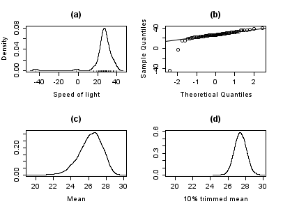
The plot below shows a density plot of the speed-of-light data, together with a rug plot (panel (a)). Also shown is a normal Q–Q plot (panel (b)). The outliers are clearly visible in these plots.

Panels (c) and (d) of the plot show the bootstrap distribution of the mean (c) and the 10% trimmed mean (d). The trimmed mean is a simple robust estimator of location that deletes a certain percentage of observations (10% here) from each end of the data, then computes the mean in the usual way. The analysis was performed in R and 10,000 bootstrap samples were used for each of the raw and trimmed means.

The distribution of the mean is clearly much wider than that of the 10% trimmed mean (the plots are on the same scale). Also note that whereas the distribution of the trimmed mean appears to be close to normal, the distribution of the raw mean is quite skewed to the left. So, in this sample of 66 observations, only 2 outliers cause the central limit theorem to be inapplicable.

Robust statistical methods, of which the trimmed mean is a simple example, seek to outperform classical statistical methods in the presence of outliers, or, more generally, when underlying parametric assumptions are not quite correct.

Whilst the trimmed mean performs well relative to the mean in this example, better robust estimates are available. In fact, the mean, median and trimmed mean are all special cases of M-estimators. Details appear in the sections below.

Estimation of scale

The outliers in the speed-of-light data have more than just an adverse effect on the mean; the usual estimate of scale is the standard deviation, and this quantity is even more badly affected by outliers because the squares of the deviations from the mean go into the calculation, so the outliers' effects are exacerbated.

The plots below show the bootstrap distributions of the standard deviation, median absolute deviation (MAD) and Qn estimator of scale.^[2] The plots are based on 10,000 bootstrap samples for each estimator, with some Gaussian noise added to the resampled data (smoothed bootstrap). Panel (a) shows the distribution of the standard deviation, (b) of the MAD and (c) of Qn.

The distribution of standard deviation is erratic and wide, a result of the outliers. The MAD is better behaved, and Qn is a little bit more efficient than MAD. This simple example demonstrates that when outliers are present, the standard deviation cannot be recommended as an estimate of scale.

Manual screening for outliers

Traditionally, statisticians would manually screen data for outliers, and remove them, usually checking the source of the data to see whether the outliers were erroneously recorded. Indeed, in the speed-of-light example above, it is easy to see and remove the two outliers prior to proceeding with any further analysis. However, in modern times, data sets often consist of large numbers of variables being measured on large numbers of experimental units. Therefore, manual screening for outliers is often impractical.

Outliers can often interact in such a way that they mask each other. As a simple example, consider a small univariate data set containing one modest and one large outlier. The estimated standard deviation will be grossly inflated by the large outlier. The result is that the modest outlier looks relatively normal. As soon as the large outlier is removed, the estimated standard deviation shrinks, and the modest outlier now looks unusual.

This problem of masking gets worse as the complexity of the data increases. For example, in regression problems, diagnostic plots are used to identify outliers. However, it is common that once a few outliers have been removed, others become visible. The problem is even worse in higher dimensions.

Robust methods provide automatic ways of detecting, downweighting (or removing), and flagging outliers, largely removing the need for manual screening. Care must be taken; initial data showing the ozone hole first appearing over Antarctica were rejected as outliers by non-human screening.^[3]

Variety of applications

Although this article deals with general principles for univariate statistical methods, robust methods also exist for regression problems, generalized linear models, and parameter estimation of various distributions.

Measures of robustness

The basic tools used to describe and measure robustness are, the breakdown point, the influence function and the sensitivity curve.

Breakdown point

Intuitively, the breakdown point of an estimator is the proportion of incorrect observations (e.g. arbitrarily large observations) an estimator can handle before giving an incorrect (e.g., arbitrarily large) result. For example, given n{displaystyle n} independent random variables (X1,…,Xn){displaystyle (X_{1},dots ,X_{n})} and the corresponding realizations x1,…,xn{displaystyle x_{1},dots ,x_{n}}, we can use Xn¯:=X1+⋯+Xnn{displaystyle {overline {X_{n}}}:={frac {X_{1}+cdots +X_{n}}{n}}} to estimate the mean. Such an estimator has a breakdown point of 0 because we can make x¯{displaystyle {overline {x}}} arbitrarily large just by changing any of x1,…,xn{displaystyle x_{1},dots ,x_{n}}.

The higher the breakdown point of an estimator, the more robust it is. Intuitively, we can understand that a breakdown point cannot exceed 50% because if more than half of the observations are contaminated, it is not possible to distinguish between the underlying distribution and the contaminating distribution Rousseeuw & Leroy (1986). Therefore, the maximum breakdown point is 0.5 and there are estimators which achieve such a breakdown point. For example, the median has a breakdown point of 0.5. The X% trimmed mean has breakdown point of X%, for the chosen level of X. Huber (1981) and Maronna, Martin & Yohai (2006) contain more details. The level and the power breakdown points of tests are investigated in He, Simpson & Portnoy (1990).

Statistics with high breakdown points are sometimes called resistant statistics.^[4]

Example: speed-of-light data

In the speed-of-light example, removing the two lowest observations causes the mean to change from 26.2 to 27.75, a change of 1.55. The estimate of scale produced by the Qn method is 6.3. We can divide this by the square root of the sample size to get a robust standard error, and we find this quantity to be 0.78. Thus, the change in the mean resulting from removing two outliers is approximately twice the robust standard error.

The 10% trimmed mean for the speed-of-light data is 27.43. Removing the two lowest observations and recomputing gives 27.67. Clearly, the trimmed mean is less affected by the outliers and has a higher breakdown point.

Notice that if we replace the lowest observation, −44, by −1000, the mean becomes 11.73, whereas the 10% trimmed mean is still 27.43. In many areas of applied statistics, it is common for data to be log-transformed to make them near symmetrical. Very small values become large negative when log-transformed, and zeroes become negatively infinite. Therefore, this example is of practical interest.

Empirical influence function

This article may be too technical for most readers to understand. Please help improve it to make it understandable to non-experts, without removing the technical details. (June 2010) (Learn how and when to remove this template message)

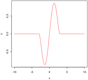
Tukey's biweight function

The empirical influence function is a measure of the dependence of the estimator on the value of one of the points in the sample. It is a model-free measure in the sense that it simply relies on calculating the estimator again with a different sample. On the right is Tukey's biweight function, which, as we will later see, is an example of what a "good" (in a sense defined later on) empirical influence function should look like.

In mathematical terms, an influence function is defined as a vector in the space of the estimator, which is in turn defined for a sample which is a subset of the population:

1. 
   (Ω,A,P){displaystyle (Omega ,{mathcal {A}},P)} is a probability space,


2. 
   (X,Σ){displaystyle ({mathcal {X}},Sigma )} is a measure space (state space),


3. 
   Θ{displaystyle Theta } is a parameter space of dimension p∈N∗{displaystyle pin mathbb {N} ^{*}},


4. 
   (Γ,S){displaystyle (Gamma ,S)} is a measure space,

For example,

1. 
   (Ω,A,P){displaystyle (Omega ,{mathcal {A}},P)} is any probability space,


2. 
   (X,Σ)=(R,B){displaystyle ({mathcal {X}},Sigma )=(mathbb {R} ,{mathcal {B}})},


3. Θ=R×R+{displaystyle Theta =mathbb {R} times mathbb {R} ^{+}}


4. 
   (Γ,S)=(R,B){displaystyle (Gamma ,S)=(mathbb {R} ,{mathcal {B}})},

The definition of an empirical influence function is:
Let n∈N∗{displaystyle nin mathbb {N} ^{*}} and X1,…,Xn:(Ω,A)→(X,Σ){displaystyle X_{1},dots ,X_{n}:(Omega ,{mathcal {A}})rightarrow ({mathcal {X}},Sigma )} are i.i.d. and (x1,…,xn){displaystyle (x_{1},dots ,x_{n})} is a sample from these variables. Tn:(Xn,Σn)→(Γ,S){displaystyle T_{n}:({mathcal {X}}^{n},Sigma ^{n})rightarrow (Gamma ,S)} is an estimator. Let i∈{1,…,n}{displaystyle iin {1,dots ,n}}. The empirical influence function EIFi{displaystyle EIF_{i}} at observation i{displaystyle i} is defined by:

EIFi:x∈X↦n⋅(Tn(x1,…,xi−1,x,xi+1,…,xn)−Tn(x1,…,xi−1,xi,xi+1,…,xn)){displaystyle EIF_{i}:xin {mathcal {X}}mapsto ncdot (T_{n}(x_{1},dots ,x_{i-1},x,x_{i+1},dots ,x_{n})-T_{n}(x_{1},dots ,x_{i-1},x_{i},x_{i+1},dots ,x_{n}))}

What this actually means is that we are replacing the i-th value in the sample by an arbitrary value and looking at the output of the estimator. Alternatively, the EIF is defined as the (scaled by n+1 instead of n) effect on the estimator of adding the point x{displaystyle x} to the sample.^{[citation needed]}

Influence function and sensitivity curve

Instead of relying solely on the data, we could use the distribution of the random variables. The approach is quite different from that of the previous paragraph. What we are now trying to do is to see what happens to an estimator when we change the distribution of the data slightly: it assumes a distribution, and measures sensitivity to change in this distribution. By contrast, the empirical influence assumes a sample set, and measures sensitivity to change in the samples.^[5]

Let A{displaystyle A} be a convex subset of the set of all finite signed measures on Σ{displaystyle Sigma }. We want to estimate the parameter θ∈Θ{displaystyle theta in Theta } of a distribution F{displaystyle F} in A{displaystyle A}. Let the functional T:A→Γ{displaystyle T:Arightarrow Gamma } be the asymptotic value of some estimator sequence (Tn)n∈N{displaystyle (T_{n})_{nin mathbb {N} }}. We will suppose that this functional is Fisher consistent, i.e. ∀θ∈Θ,T(Fθ)=θ{displaystyle forall theta in Theta ,T(F_{theta })=theta }. This means that at the model F{displaystyle F}, the estimator sequence asymptotically measures the correct quantity.

Let G{displaystyle G} be some distribution in A{displaystyle A}. What happens when the data doesn't follow the model F{displaystyle F} exactly but another, slightly different, "going towards" G{displaystyle G}?

We're looking at: dTG−F(F)=limt→0+T(tG+(1−t)F)−T(F)t{displaystyle dT_{G-F}(F)=lim _{trightarrow 0^{+}}{frac {T(tG+(1-t)F)-T(F)}{t}}},

which is the one-sided directional derivative of T{displaystyle T} at F{displaystyle F}, in the direction of G−F{displaystyle G-F}.

Let x∈X{displaystyle xin {mathcal {X}}}. Δx{displaystyle Delta _{x}} is the probability measure which gives mass 1 to {x}{displaystyle {x}}. We choose G=Δx{displaystyle G=Delta _{x}}. The influence function is then defined by:

IF(x;T;F):=limt→0+T(tΔx+(1−t)F)−T(F)t.{displaystyle IF(x;T;F):=lim _{trightarrow 0^{+}}{frac {T(tDelta _{x}+(1-t)F)-T(F)}{t}}.}

It describes the effect of an infinitesimal contamination at the point x{displaystyle x} on the estimate we are seeking, standardized by the mass t{displaystyle t} of the contamination (the asymptotic bias caused by contamination in the observations). For a robust estimator, we want a bounded influence function, that is, one which does not go to infinity as x becomes arbitrarily large.

Desirable properties

Properties of an influence function which bestow it with desirable performance are:

1. Finite rejection point ρ∗{displaystyle rho ^{*}},


2. Small gross-error sensitivity γ∗{displaystyle gamma ^{*}},


3. Small local-shift sensitivity λ∗{displaystyle lambda ^{*}}.

Rejection point

ρ∗:=infr>0{r:IF(x;T;F)=0,|x|>r}{displaystyle rho ^{*}:=inf _{r>0}{r:IF(x;T;F)=0,|x|>r}}

Gross-error sensitivity

γ∗(T;F):=supx∈X|IF(x;T;F)|{displaystyle gamma ^{*}(T;F):=sup _{xin {mathcal {X}}}|IF(x;T;F)|}

Local-shift sensitivity

λ∗(T;F):=sup(x,y)∈X2x≠y‖IF(y;T;F)−IF(x;T;F)y−x‖{displaystyle lambda ^{*}(T;F):=sup _{(x,y)in {mathcal {X}}^{2} atop xneq y}left|{frac {IF(y;T;F)-IF(x;T;F)}{y-x}}right|}

This value, which looks a lot like a Lipschitz constant, represents the effect of shifting an observation slightly from x{displaystyle x} to a neighbouring point y{displaystyle y}, i.e., add an observation at y{displaystyle y} and remove one at x{displaystyle x}.

M-estimators

(The mathematical context of this paragraph is given in the section on empirical influence functions.)

Historically, several approaches to robust estimation were proposed, including R-estimators and L-estimators. However, M-estimators now appear to dominate the field as a result of their generality, high breakdown point, and their efficiency. See Huber (1981).

M-estimators are a generalization of maximum likelihood estimators (MLEs). What we try to do with MLE's is to maximize ∏i=1nf(xi){displaystyle prod _{i=1}^{n}f(x_{i})} or, equivalently, minimize ∑i=1n−log⁡f(xi){displaystyle sum _{i=1}^{n}-log f(x_{i})}. In 1964, Huber proposed to generalize this to the minimization of ∑i=1nρ(xi){displaystyle sum _{i=1}^{n}rho (x_{i})}, where ρ{displaystyle rho } is some function. MLE are therefore a special case of M-estimators (hence the name: "Maximum likelihood type" estimators).

Minimizing ∑i=1nρ(xi){displaystyle sum _{i=1}^{n}rho (x_{i})} can often be done by differentiating ρ{displaystyle rho } and solving ∑i=1nψ(xi)=0{displaystyle sum _{i=1}^{n}psi (x_{i})=0}, where ψ(x)=dρ(x)dx{displaystyle psi (x)={frac {drho (x)}{dx}}} (if ρ{displaystyle rho } has a derivative).

Several choices of ρ{displaystyle rho } and ψ{displaystyle psi } have been proposed. The two figures below show four ρ{displaystyle rho } functions and their corresponding ψ{displaystyle psi } functions.

For squared errors, ρ(x){displaystyle rho (x)} increases at an accelerating rate, whilst for absolute errors, it increases at a constant rate. When Winsorizing is used, a mixture of these two effects is introduced: for small values of x, ρ{displaystyle rho } increases at the squared rate, but once the chosen threshold is reached (1.5 in this example), the rate of increase becomes constant. This Winsorised estimator is also known as the Huber loss function.

Tukey's biweight (also known as bisquare) function behaves in a similar way to the squared error function at first, but for larger errors, the function tapers off.

Properties of M-estimators

Notice that M-estimators do not necessarily relate to a probability density function. Therefore, off-the-shelf approaches to inference that arise from likelihood theory can not, in general, be used.

It can be shown that M-estimators are asymptotically normally distributed, so that as long as their standard errors can be computed, an approximate approach to inference is available.

Since M-estimators are normal only asymptotically, for small sample sizes it might be appropriate to use an alternative approach to inference, such as the bootstrap. However, M-estimates are not necessarily unique (i.e., there might be more than one solution that satisfies the equations). Also, it is possible that any particular bootstrap sample can contain more outliers than the estimator's breakdown point. Therefore, some care is needed when designing bootstrap schemes.

Of course, as we saw with the speed-of-light example, the mean is only normally distributed asymptotically and when outliers are present the approximation can be very poor even for quite large samples. However, classical statistical tests, including those based on the mean, are typically bounded above by the nominal size of the test. The same is not true of M-estimators and the type I error rate can be substantially above the nominal level.

These considerations do not "invalidate" M-estimation in any way. They merely make clear that some care is needed in their use, as is true of any other method of estimation.

Influence function of an M-estimator

It can be shown that the influence function of an M-estimator T{displaystyle T} is proportional to ψ{displaystyle psi },^[6] which means we can derive the properties of such an estimator (such as its rejection point, gross-error sensitivity or local-shift sensitivity) when we know its ψ{displaystyle psi } function.

IF(x;T,F)=M−1ψ(x,T(F)){displaystyle IF(x;T,F)=M^{-1}psi (x,T(F))}

with the p×p{displaystyle ptimes p} given by:

M=−∫X(∂ψ(x,θ)∂θ)T(F)dF(x).{displaystyle M=-int _{mathcal {X}}left({frac {partial psi (x,theta )}{partial theta }}right)_{T(F)},dF(x).}

Choice of ψ and ρ

In many practical situations, the choice of the ψ{displaystyle psi } function is not critical to gaining a good robust estimate, and many choices will give similar results that offer great improvements, in terms of efficiency and bias, over classical estimates in the presence of outliers.^[7]

Theoretically, ψ{displaystyle psi } functions are to be preferred, and Tukey's biweight (also known as bisquare) function is a popular choice. Maronna, Martin & Yohai (2006) recommend the biweight function with efficiency at the normal set to 85%.

Robust parametric approaches

M-estimators do not necessarily relate to a density function and so are not fully parametric. Fully parametric approaches to robust modeling and inference, both Bayesian and likelihood approaches, usually deal with heavy tailed distributions such as Student's t-distribution.

For the t-distribution with ν{displaystyle nu } degrees of freedom, it can be shown that

ψ(x)=xx2+ν.{displaystyle psi (x)={frac {x}{x^{2}+nu }}.}

For ν=1{displaystyle nu =1}, the t-distribution is equivalent to the Cauchy distribution. Notice that the degrees of freedom is sometimes known as the kurtosis parameter. It is the parameter that controls how heavy the tails are. In principle, ν{displaystyle nu } can be estimated from the data in the same way as any other parameter. In practice, it is common for there to be multiple local maxima when ν{displaystyle nu } is allowed to vary. As such, it is common to fix ν{displaystyle nu } at a value around 4 or 6. The figure below displays the ψ{displaystyle psi }-function for 4 different values of ν{displaystyle nu }.

Example: speed-of-light data

For the speed-of-light data, allowing the kurtosis parameter to vary and maximizing the likelihood, we get

μ^=27.40,σ^=3.81,ν^=2.13.{displaystyle {hat {mu }}=27.40,{hat {sigma }}=3.81,{hat {nu }}=2.13.}

Fixing ν=4{displaystyle nu =4} and maximizing the likelihood gives

μ^=27.49,σ^=4.51.{displaystyle {hat {mu }}=27.49,{hat {sigma }}=4.51.}

Related concepts

A pivotal quantity is a function of data, whose underlying population distribution is a member of a parametric family, that is not dependent on the values of the parameters. An ancillary statistic is such a function that is also a statistic, meaning that it is computed in terms of the data alone. Such functions are robust to parameters in the sense that they are independent of the values of the parameters, but not robust to the model in the sense that they assume an underlying model (parametric family), and in fact such functions are often very sensitive to violations of the model assumptions. Thus test statistics, frequently constructed in terms of these to not be sensitive to assumptions about parameters, are still very sensitive to model assumptions.

Replacing outliers and missing values

Replacing missing data is called imputation. If there are relatively few missing points, there are some models which can be used to estimate values to complete the series, such as replacing missing values with the mean or median of the data. Simple linear regression can also be used to estimate missing values.^[8] In addition, outliers can sometimes be accommodated in the data through the use of trimmed means, other scale estimators apart from standard deviation (e.g., MAD) and Winsorization.^[9] In calculations of a trimmed mean, a fixed percentage of data is dropped from each end of an ordered data, thus eliminating the outliers. The mean is then calculated using the remaining data. Winsorizing involves accommodating an outlier by replacing it with the next highest or next smallest value as appropriate.^[10]

However, using these types of models to predict missing values or outliers in a long time series is difficult and often unreliable, particularly if the number of values to be in-filled is relatively high in comparison with total record length. The accuracy of the estimate depends on how good and representative the model is and how long the period of missing values extends.^[11] The in a case of a dynamic process, so any variable is dependent, not just on the historical time series of the same variable but also on several other variables or parameters of the process. In other words, the problem is an exercise in multivariate analysis rather than the univariate approach of most of the traditional methods of estimating missing values and outliers; a multivariate model will therefore be more representative than a univariate one for predicting missing values. The Kohonen self organising map (KSOM) offers a simple and robust multivariate model for data analysis, thus providing good possibilities to estimate missing values, taking into account its relationship or correlation with other pertinent variables in the data record.^[10]

Standard Kalman filters are not robust to outliers. To this end Ting, Theodorou & Schaal (2007) have recently shown that a modification of Masreliez's theorem can deal with outliers.

One common approach to handle outliers in data analysis is to perform outlier detection first, followed by an efficient estimation method (e.g., the least squares). While this approach is often useful, one must keep in mind two challenges. First, an outlier detection method that relies on a non-robust initial fit can suffer from the effect of masking, that is, a group of outliers can mask each other and escape detection.^[12] Second, if a high breakdown initial fit is used for outlier detection, the follow-up analysis might inherit some of the inefficiencies of the initial estimator.^[13]

See also

• Robust confidence intervals


• Robust regression


• Unit-weighted regression


• Imputation (statistics)

Notes

References

• 
  Hampel, Frank R.; Ronchetti, Elvezio M.; Rousseeuw, Peter J.; Stahel, Werner A. (1986), Robust statistics, Wiley Series in Probability and Mathematical Statistics: Probability and Mathematical Statistics, New York: John Wiley & Sons, Inc., ISBN 0-471-82921-8, MR 0829458.mw-parser-output cite.citation{font-style:inherit}.mw-parser-output q{quotes:"""""""'""'"}.mw-parser-output code.cs1-code{color:inherit;background:inherit;border:inherit;padding:inherit}.mw-parser-output .cs1-lock-free a{background:url("//upload.wikimedia.org/wikipedia/commons/thumb/6/65/Lock-green.svg/9px-Lock-green.svg.png")no-repeat;background-position:right .1em center}.mw-parser-output .cs1-lock-limited a,.mw-parser-output .cs1-lock-registration a{background:url("//upload.wikimedia.org/wikipedia/commons/thumb/d/d6/Lock-gray-alt-2.svg/9px-Lock-gray-alt-2.svg.png")no-repeat;background-position:right .1em center}.mw-parser-output .cs1-lock-subscription a{background:url("//upload.wikimedia.org/wikipedia/commons/thumb/a/aa/Lock-red-alt-2.svg/9px-Lock-red-alt-2.svg.png")no-repeat;background-position:right .1em center}.mw-parser-output .cs1-subscription,.mw-parser-output .cs1-registration{color:#555}.mw-parser-output .cs1-subscription span,.mw-parser-output .cs1-registration span{border-bottom:1px dotted;cursor:help}.mw-parser-output .cs1-hidden-error{display:none;font-size:100%}.mw-parser-output .cs1-visible-error{font-size:100%}.mw-parser-output .cs1-subscription,.mw-parser-output .cs1-registration,.mw-parser-output .cs1-format{font-size:95%}.mw-parser-output .cs1-kern-left,.mw-parser-output .cs1-kern-wl-left{padding-left:0.2em}.mw-parser-output .cs1-kern-right,.mw-parser-output .cs1-kern-wl-right{padding-right:0.2em}. Republished in paperback, 2005.


• 
  He, Xuming; Portnoy, Stephen (1992), "Reweighted LS estimators converge at the same rate as the initial estimator", Annals of Statistics, 20 (4): 2161–2167, doi:10.1214/aos/1176348910, MR 1193333.


• 
  He, Xuming; Simpson, Douglas G.; Portnoy, Stephen L. (1990), "Breakdown robustness of tests", Journal of the American Statistical Association, 85 (410): 446–452, doi:10.2307/2289782, MR 1141746.


• 
  Hettmansperger, T. P.; McKean, J. W. (1998), Robust nonparametric statistical methods, Kendall's Library of Statistics, 5, New York: John Wiley & Sons, Inc., ISBN 0-340-54937-8, MR 1604954. 2nd ed., CRC Press, 2011.


• 
  Huber, Peter J. (1981), Robust statistics, New York: John Wiley & Sons, Inc., ISBN 0-471-41805-6, MR 0606374. Republished in paperback, 2004. 2nd ed., Wiley, 2009.


• 
  MacDonald, Iain L.; Zucchini, Walter (1997), Hidden Markov and other models for discrete-valued time series, Monographs on Statistics and Applied Probability, 70, London: Chapman & Hall, ISBN 0-412-55850-5, MR 1692202.


• 
  Maronna, Ricardo A.; Martin, R. Douglas; Yohai, Victor J. (2006), Robust statistics: Theory and methods, Wiley Series in Probability and Statistics, Chichester: John Wiley & Sons, Ltd., doi:10.1002/0470010940, ISBN 978-0-470-01092-1, MR 2238141.


• 
  McBean, Edward A.; Rovers, Frank (1998), Statistical procedures for analysis of environmental monitoring data and assessment, Prentice-Hall.


• 
  Portnoy, Stephen; He, Xuming (2000), "A robust journey in the new millennium", Journal of the American Statistical Association, 95 (452): 1331–1335, doi:10.2307/2669782, MR 1825288.


• 
  Press, William H.; Teukolsky, Saul A.; Vetterling, William T.; Flannery, Brian P. (2007), "Section 15.7. Robust Estimation", Numerical Recipes: The Art of Scientific Computing (3rd ed.), Cambridge University Press, ISBN 978-0-521-88068-8, MR 2371990.


• 
  Rosen, C.; Lennox, J.A. (October 2001), "Multivariate and multiscale monitoring of wastewater treatment operation", Water Research, 35 (14): 3402–3410, doi:10.1016/s0043-1354(01)00069-0.


• 
  Rousseeuw, Peter J.; Croux, Christophe (1993), "Alternatives to the median absolute deviation", Journal of the American Statistical Association, 88 (424): 1273–1283, doi:10.2307/2291267, MR 1245360.


• 
  Rousseeuw, Peter J.; Leroy, Annick M. (1987), Robust regression and outlier detection, Wiley Series in Probability and Mathematical Statistics: Applied Probability and Statistics, New York: John Wiley & Sons, Inc., doi:10.1002/0471725382, ISBN 0-471-85233-3, MR 0914792. Republished in paperback, 2003.


• 
  Rousseeuw, Peter J.; Hubert, Mia (2011), "Robust statistics for outlier detection", Wiley Interdisciplinary Reviews: Data Mining and Knowledge Discovery (1): 73–79, doi:10.1002/widm.2. Preprint
  


• 
  Rustum, Rabee; Adeloye, Adebayo J. (September 2007), "Replacing outliers and missing values from activated sludge data using Kohonen self-organizing map", Journal of Environmental Engineering, 133 (9): 909–916, doi:10.1061/(asce)0733-9372(2007)133:9(909).


• 
  Stigler, Stephen M. (2010), "The changing history of robustness", The American Statistician, 64 (4): 277–281, doi:10.1198/tast.2010.10159, MR 2758558.


• 
  Ting, Jo-anne; Theodorou, Evangelos; Schaal, Stefan (2007), "A Kalman filter for robust outlier detection", International Conference on Intelligent Robots and Systems – IROS, pp. 1514–1519.


• 
  von Mises, R. (1947), "On the asymptotic distribution of differentiable statistical functions", Annals of Mathematical Statistics, 18: 309–348, doi:10.1214/aoms/1177730385, MR 0022330.


• 
  Wilcox, Rand (2012), Introduction to robust estimation and hypothesis testing, Statistical Modeling and Decision Science (3rd ed.), Amsterdam: Elsevier/Academic Press, pp. 1–22, doi:10.1016/B978-0-12-386983-8.00001-9, ISBN 978-0-12-386983-8, MR 3286430.

External links

• 
  Brian Ripley's robust statistics course notes.
  


• 
  Nick Fieller's course notes on Statistical Modelling and Computation contain material on robust regression.


• 
  David Olive's site contains course notes on robust statistics and some data sets.


• Online experiments using R and JSXGraph